Tutorials
End-to-end examples, ordered roughly from simplest to most involved. Each defines a model as an @latte function (or a plain DPPL @model) and runs it through one of Latte's inference engines: inla, tmb, or hmc_laplace.
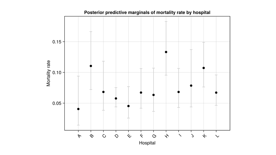
Surgery mortality across hospitals
Hospital-by-hospital surgery mortality with an IID random effect, written once and run through all three engines (INLA, TMB, HMC-Laplace) in a few lines each.
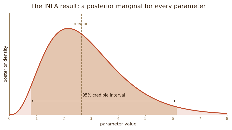
Getting familiar with INLA
Stay with the surgery model and dig into the INLA result object: reading marginals through the accessor functions, the model-comparison criteria (DIC, WAIC, marginal likelihood), and joint posterior sampling.
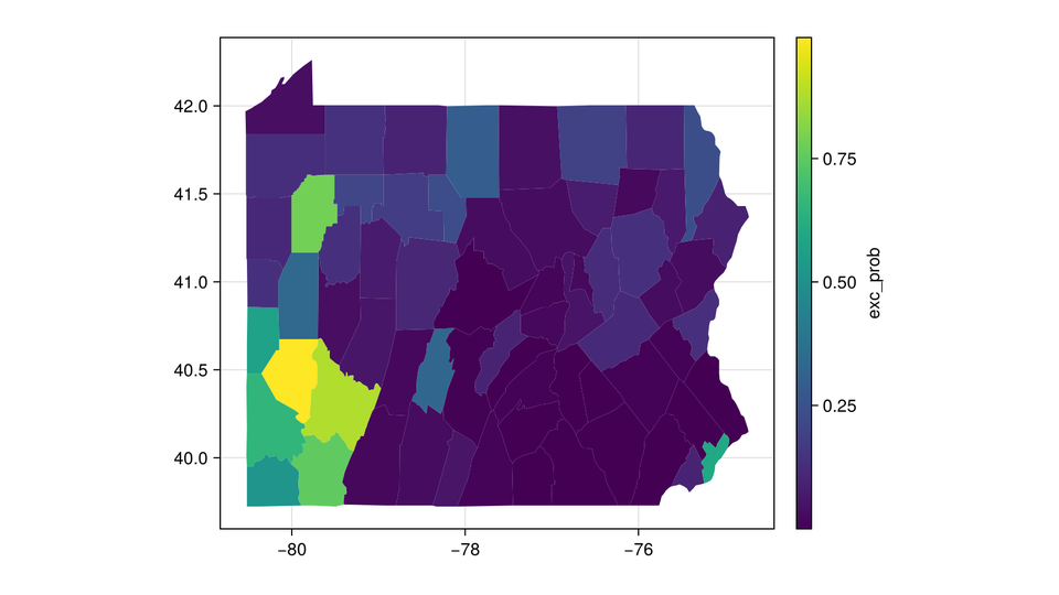
BYM: Besag + IID
Regional disease risk smoothed with an ICAR spatial prior plus an IID residual. PC priors on both precisions, fit with INLA.
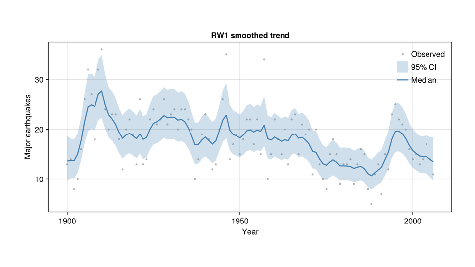
Earthquake intensity trends
RW1 vs RW2 priors on annual seismicity counts, compared by DIC, WAIC, and marginal likelihood — all from the same fit object.
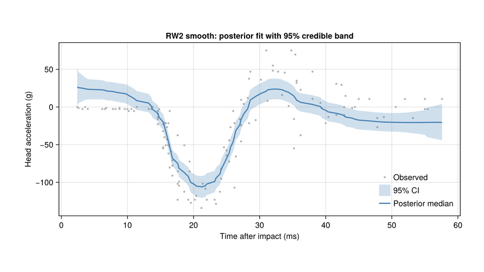
Nonlinear regression with RW2
A generalised-additive-model take on a smooth regression: an RW2 prior on the latent function, Gaussian likelihood.
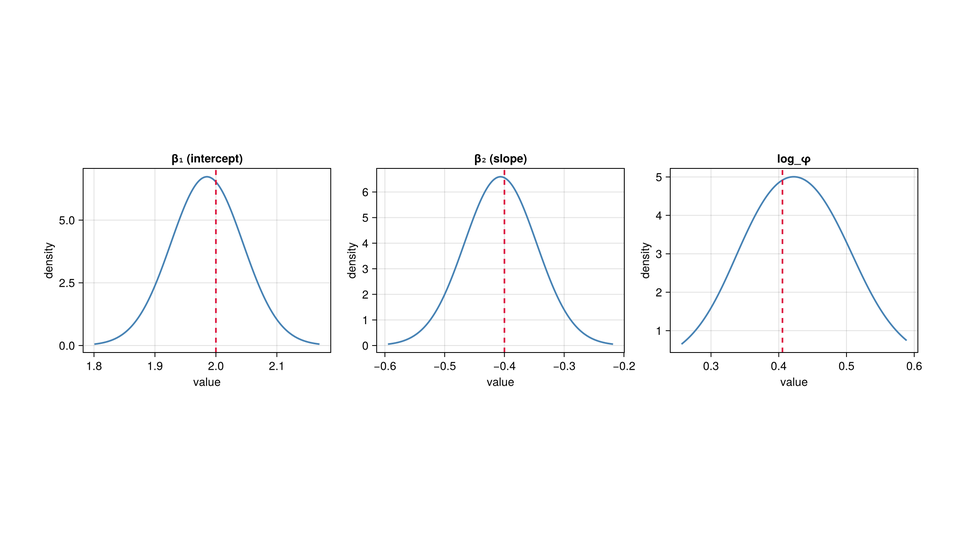
Tweedie regression on insurance claims
Write any logpdf, get full INLA inference. A hand-coded compound Poisson-Gamma likelihood — zero-inflated continuous, no fast-path support — fits in the same DPPL @model + inla() flow.
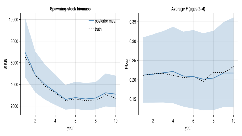
Age-structured stock assessment (SAM)
The Nielsen & Berg assessment model: coupled log-numbers and log-fishing-mortality fields with a nonlinear survival recursion. @latte recognises the non-Gaussian latent prior from the ~ statements and fits it by iterated Laplace.
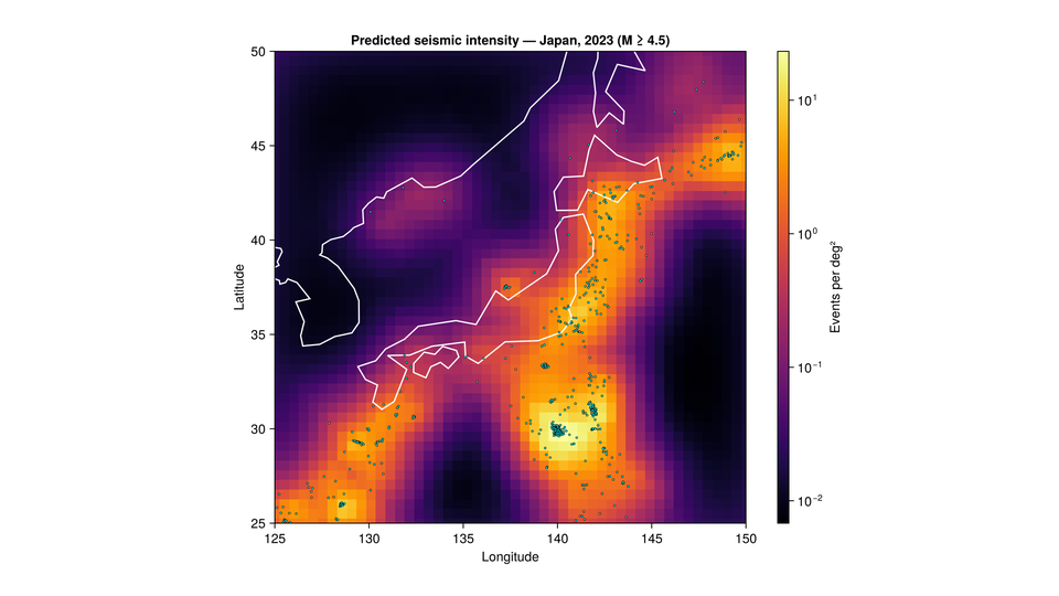
Matérn SPDE on a mesh
Continuous-domain spatial smoothing via the SPDE/Matérn approach. Build a triangulated mesh, define the Matérn precision, fit.
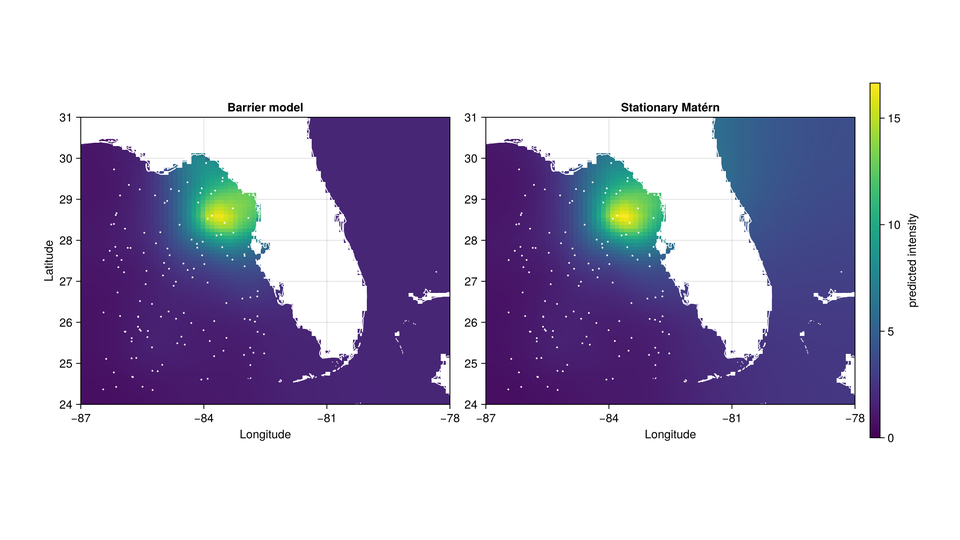
Spatial fields that respect coastlines
A stationary Matérn field smooths fish abundance straight across the Florida peninsula; a barrier model (Bakka et al.) does not. Same LGCP, swap the prior, and the phantom hot spot across the peninsula disappears.
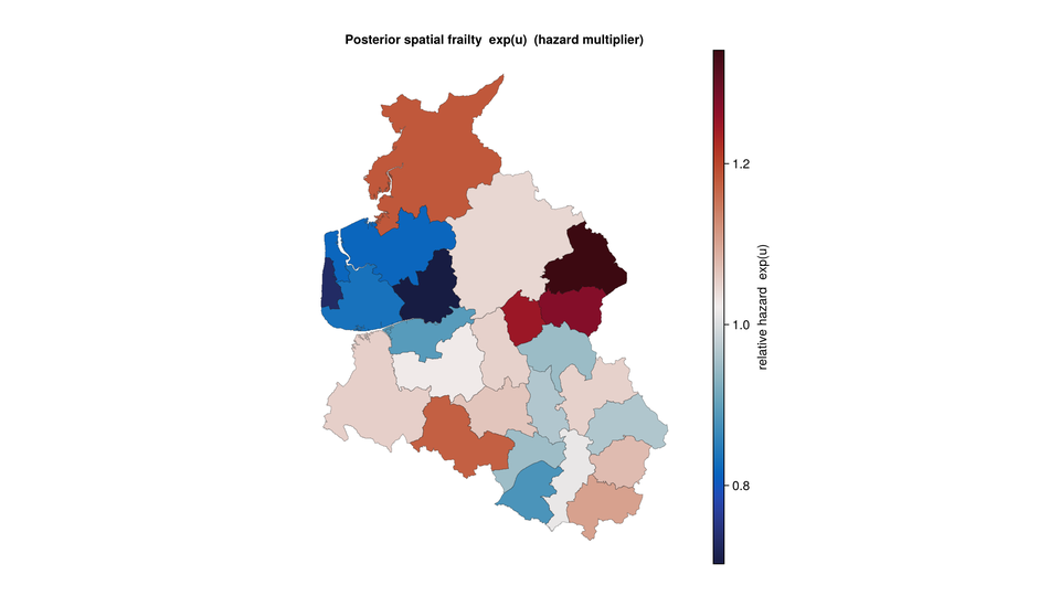
Spatial survival: leukemia hazards
Time-to-event with right-censoring and a Besag spatial frailty over 24 districts, fit two ways: the Poisson piecewise-exponential trick on the fast path, and a hand-written Weibull likelihood. Both agree with each other and with R-INLA.
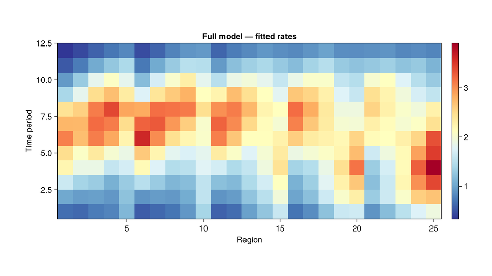
Kronecker space-time
Region-specific temporal dynamics via a SeparableModel Kronecker prior. Additive vs interaction-only vs full, on one DPPL spec.
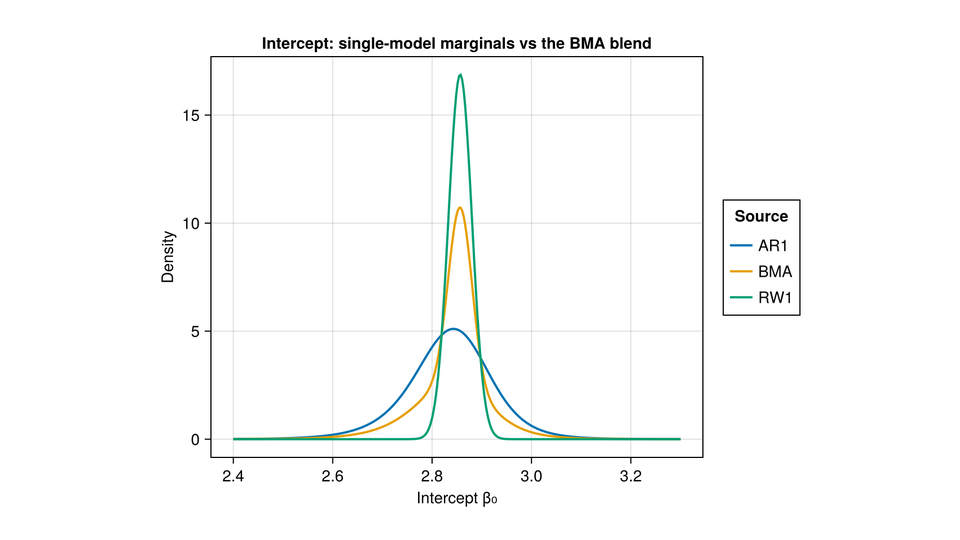
Bayesian model averaging
Two competing trend models (RW1 vs AR1) on annual earthquake counts, with near-tied marginal likelihoods. Their posterior weights come out close to even, so the averaged trend is a genuine blend.
Posterior predictive checks
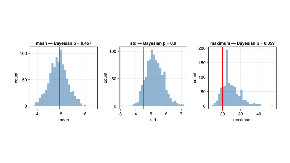
Catch model misspecification by simulating from the fitted posterior. A Poisson model fitted to overdispersed counts, exposed by a `std` PPC.
Simulation-based calibration
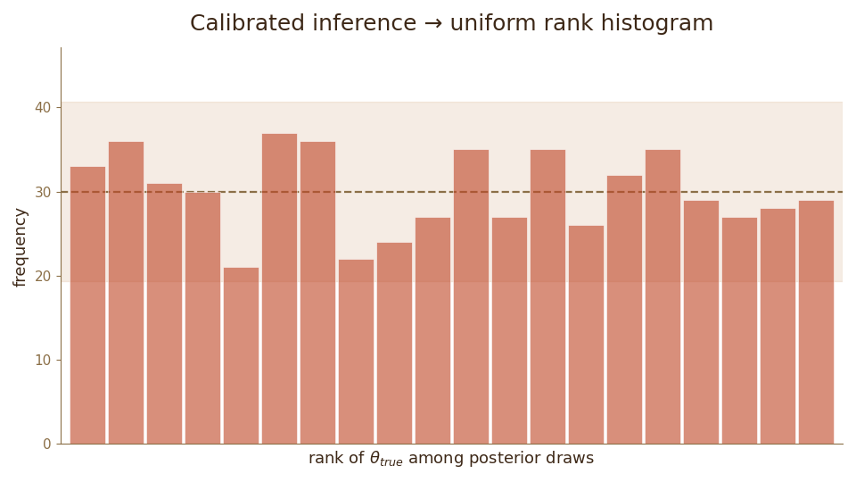
Validate the inference procedure itself: rank true parameters in the posterior across many simulated datasets. Uniform ranks ⇒ calibrated.
Handoff to Turing
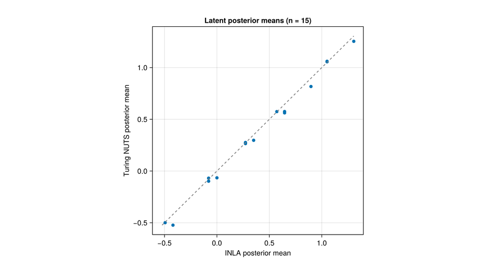
The same DPPL @model that fits with INLA also samples cleanly under Turing.sample(NUTS()). Use it as a gold-standard cross-check.
When to sample the hyperparameters
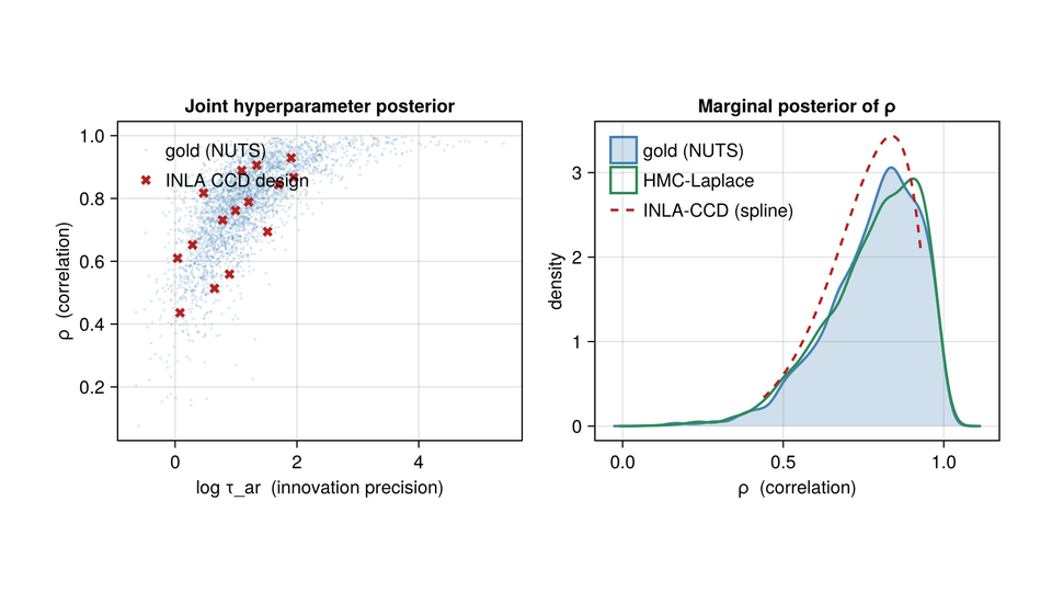
INLA integrates the hyperparameters out on a deterministic grid; when that posterior is a curved, skewed ridge, the design is biased. hmc_laplace samples it instead — shown on an AR(1) model, validated against gold-standard NUTS.