Temporal trend smoothing: Global earthquake activity

Raw counts of rare events are noisy. Is the number of major earthquakes really changing over time, or are we just seeing random fluctuation? Here we use INLA with random walk models to smooth annual earthquake counts and look for a long-term trend.

The tutorial covers a Poisson model with a temporal random effect, the difference between first- and second-order random walks (RW1 and RW2), the role of the random-walk precision in controlling smoothness, and model comparison via DIC and WAIC.

The dataset

We use annual counts of major earthquakes (magnitude $\geq$ 7) from 1900 to 2006. This dataset appears in Zucchini et al. (2016) and the INLA gitbook. With 107 observations it fits in a single code block:

julia

using DataFrames
quake_counts = [
    13, 14, 8, 10, 16, 26, 32, 27, 18, 32, 36, 24, 20, 23, 23, 18, 12,
    20, 22, 19, 13, 26, 13, 14, 22, 24, 21, 22, 26, 21, 23, 24, 20, 24, 24, 22,
    20, 10, 14, 19, 23, 18, 12, 13, 20, 26, 35, 14, 17, 19, 15, 18, 22, 22, 17,
    22, 15, 34, 10, 15, 22, 18, 15, 20, 13, 22, 23, 15, 21, 19, 20, 11, 20, 13,
    10, 8, 15, 18, 15, 9, 13, 13, 14, 9, 13, 16, 15, 8, 5, 11, 13, 7, 15, 12, 23,
    25, 22, 21, 20, 16, 14, 15, 13, 14, 17, 14, 11,
]
eq_data = DataFrame(year = 1900:2006, quakes = quake_counts)
first(eq_data, 5)

5×2 DataFrame
 Row │ year   quakes
     │ Int64  Int64
─────┼───────────────
   1 │  1900      13
   2 │  1901      14
   3 │  1902       8
   4 │  1903      10
   5 │  1904      16

Let's take a first look:

julia

using AlgebraOfGraphics, CairoMakie
draw(
    data(eq_data) *
        mapping(:year => "Year", :quakes => "Major earthquakes (M ≥ 7)") *
        visual(Scatter, markersize = 5, color = :gray40),
    axis = (title = "Annual counts of major earthquakes, 1900–2006",)
)

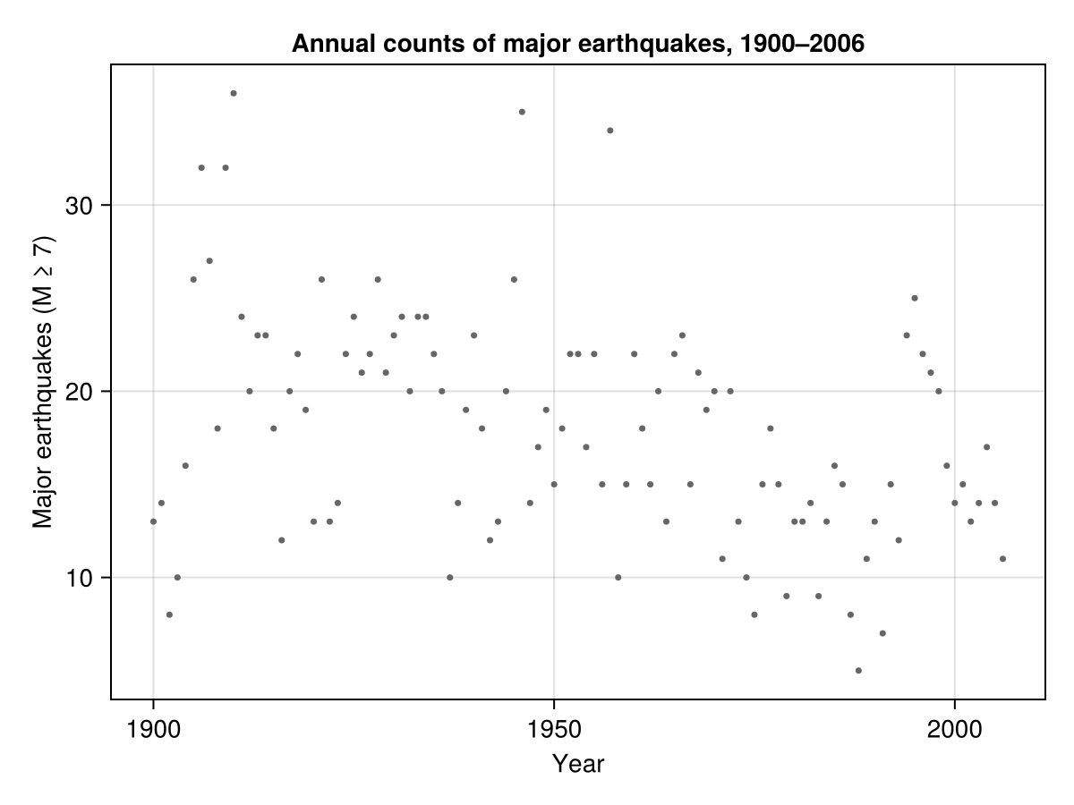
The counts bounce around a lot year to year. There seems to be a broad hump in the early-to-mid 20th century and perhaps a decline toward the end, but by eye it is hard to separate signal from noise. Temporal smoothing is one way to make that separation explicit.

Poisson model with a first-order random walk (RW1)

We model the annual count $y_{t}$ as

y_{t} \sim Poisson (λ_{t}), \log λ_{t} = β_{0} + f_{t}

where $β_{0}$ is an intercept (overall log-rate) and $f_{t}$ is a latent temporal effect. For the RW1 model, the first differences of $f$ are i.i.d. Gaussian:

f_{t + 1} - f_{t} \sim N (0, τ^{- 1})

This penalises abrupt jumps. The precision $τ$ controls the smoothness: high $τ$ means small differences (smooth trend), low $τ$ allows more wiggle (follows the data closely).

We express this as an @latte model. The random-walk prior comes from GaussianMarkovRandomFields.jl's RWModel{Order}, which we call with (τ = τ_rw) to produce a GMRF prior that @latte recognizes as a structured Gaussian. We write one model per order: RWModel{1} here, RWModel{2} below.

julia

using Latte
using Distributions
using GaussianMarkovRandomFields: RWModel
using LinearAlgebra

@latte function quake_rw1(y, n)
    τ_rw ~ PCPrior.Precision(1.0, α = 0.01)
    β ~ MvNormal(zeros(1), 100.0 * I(1))
    f ~ RWModel{1}(n)(τ = τ_rw)
    for i in eachindex(y)
        y[i] ~ Poisson(exp(β[1] + f[i]))
    end
end

quake_rw1 (generic function with 1 method)

The PC prior PCPrior.Precision(1.0, α = 0.01) says "I believe there is only a 1% chance that the standard deviation of the first differences exceeds 1".

Now we build the LatentGaussianModel (by calling the @latte function) and run INLA:

julia

n_years = nrow(eq_data)
lgm_rw1 = quake_rw1(eq_data.quakes, n_years)
result_rw1 = inla(lgm_rw1, eq_data.quakes; progress = false)

INLAResult:
  Model: LatentGaussianModel{HyperparameterSpec{@NamedTuple{τ_rw::Hyperparameter{Bijectors.TruncatedBijector{Float64, Float64}, :natural}}, @NamedTuple{}}, Latte._PatternAugmentedLatentModel{Latte.RoutedLatentModel{CombinedModel{LinearSolve.CHOLMODFactorization{Nothing}}, @NamedTuple{τ_rw1::Symbol}}, SparseArrays.SparseMatrixCSC{Int64, Int64}}, LinearlyTransformedObservationModel{ExponentialFamily{Distributions.Poisson, LogLink, Nothing, Nothing}, SparseArrays.SparseMatrixCSC{Float64, Int64}, Nothing}}
  Hyperparameters: 1
  Latent variables: 108
  Mode: (τ_rw=63.8428)
  Convergence: ✓
  Total time: 3.72 seconds
  Exploration: 5 points (5 integration)

Model comparison metrics:
Deviance Information Criterion (DIC):
  DIC: 586.91
  Effective parameters (p_D): 0.96
  Mean deviance (D̄): 585.95
  Deviance at mode: 584.98

Marginal Log-Likelihood:
  log p(y): -338.89

Watanabe-Akaike Information Criterion (WAIC):
  WAIC: 634.46
  Effective parameters (p_WAIC): 20.97
  Log pointwise predictive density (lppd): -296.26

Conditional Predictive Ordinates (CPO):
  LPML: -312.34
  Mean CPO: 0.0643
  Min CPO: 0.0004
  PIT computed: 107 values
  PIT mean: 0.5014 (ideal: 0.5)


Approximation quality (KLD):
  Max SKLD: 0.0516 (variable 1)
  Mean SKLD: 0.0005

Use .hyperparameter_marginals, .latent_marginals, .accumulators for analysis

Let's look at the fitted trend. The observation marginals give the posterior distribution of $λ_{t} = \exp (η_{t})$ , the expected count per year:

julia

obs_rw1 = observation_marginals(result_rw1)
fit_rw1 = summary_df(obs_rw1)
fit_rw1.year = eq_data.year
first(fit_rw1, 5)

5×7 DataFrame
 Row │ mode     median   q2_5      q97_5    mean     std      year
     │ Float64  Float64  Float64   Float64  Float64  Float64  Int64
─────┼──────────────────────────────────────────────────────────────
   1 │ 13.3128  13.5857   9.63899  18.6532  13.7299  2.30323   1900
   2 │ 13.484   13.6892  10.0868   18.1156  13.7955  2.05147   1901
   3 │ 13.5649  13.7148  10.1217   17.9131  13.7926  1.99078   1902
   4 │ 14.8777  15.008   11.3001   19.2604  15.0776  2.03102   1903
   5 │ 17.5398  17.7259  13.8585   22.3683  17.8256  2.16707   1904

Overlaying the posterior median and 95% interval on the raw counts:

julia

fig = Figure(size = (800, 400))
ax = Axis(
    fig[1, 1],
    xlabel = "Year", ylabel = "Major earthquakes",
    title = "RW1 smoothed trend"
)
scatter!(ax, eq_data.year, eq_data.quakes, color = :gray70, markersize = 5, label = "Observed")
band!(ax, fit_rw1.year, fit_rw1.q2_5, fit_rw1.q97_5, color = (:steelblue, 0.25), label = "95% CI")
lines!(ax, fit_rw1.year, fit_rw1.median, color = :steelblue, linewidth = 2, label = "Median")
axislegend(ax, position = :rt, framevisible = false)
fig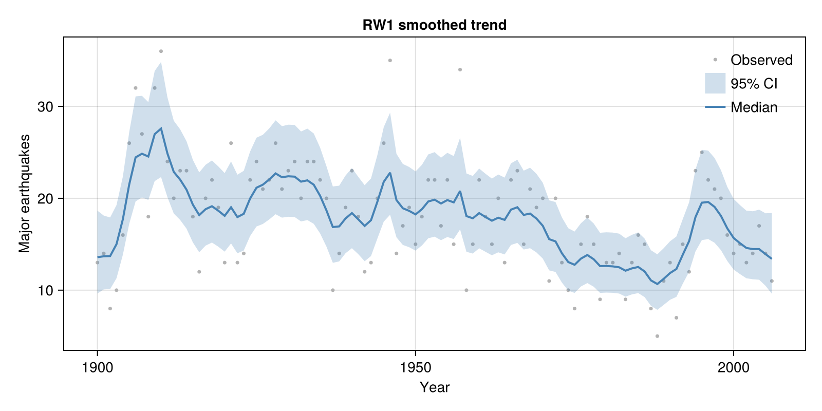

The RW1 trend is fairly wiggly and tracks local fluctuations in the data. This is characteristic of a first-order random walk: it penalises abrupt jumps in level, but changing direction from year to year carries little cost.

Poisson model with a second-order random walk (RW2)

The RW2 model penalises second differences instead:

f_{t + 2} - 2 f_{t + 1} + f_{t} \sim N (0, τ^{- 1})

This penalises changes in slope rather than changes in level, producing smoother, more slowly varying trends. The RW2 model is the same body with RWModel{2}:

julia

@latte function quake_rw2(y, n)
    τ_rw ~ PCPrior.Precision(1.0, α = 0.01)
    β ~ MvNormal(zeros(1), 100.0 * I(1))
    f ~ RWModel{2}(n)(τ = τ_rw)
    for i in eachindex(y)
        y[i] ~ Poisson(exp(β[1] + f[i]))
    end
end

lgm_rw2 = quake_rw2(eq_data.quakes, n_years)
result_rw2 = inla(lgm_rw2, eq_data.quakes; progress = false)

INLAResult:
  Model: LatentGaussianModel{HyperparameterSpec{@NamedTuple{τ_rw::Hyperparameter{Bijectors.TruncatedBijector{Float64, Float64}, :natural}}, @NamedTuple{}}, Latte._PatternAugmentedLatentModel{Latte.RoutedLatentModel{CombinedModel{LinearSolve.CHOLMODFactorization{Nothing}}, @NamedTuple{τ_rw2::Symbol}}, SparseArrays.SparseMatrixCSC{Int64, Int64}}, LinearlyTransformedObservationModel{ExponentialFamily{Distributions.Poisson, LogLink, Nothing, Nothing}, SparseArrays.SparseMatrixCSC{Float64, Int64}, Nothing}}
  Hyperparameters: 1
  Latent variables: 108
  Mode: (τ_rw=835.7721)
  Convergence: ✓
  Total time: 14.77 seconds
  Exploration: 16 points (16 integration)

Model comparison metrics:
Deviance Information Criterion (DIC):
  DIC: 646.1
  Effective parameters (p_D): 0.74
  Mean deviance (D̄): 645.36
  Deviance at mode: 644.63

Marginal Log-Likelihood:
  log p(y): -358.81

Watanabe-Akaike Information Criterion (WAIC):
  WAIC: 679.73
  Effective parameters (p_WAIC): 19.72
  Log pointwise predictive density (lppd): -320.14

Conditional Predictive Ordinates (CPO):
  LPML: -333.09
  Mean CPO: 0.0604
  Min CPO: 0.0002
  PIT computed: 107 values
  PIT mean: 0.4901 (ideal: 0.5)


Approximation quality (KLD):
  Max SKLD: 0.0148 (variable 1)
  Mean SKLD: 0.0002

Use .hyperparameter_marginals, .latent_marginals, .accumulators for analysis

And the fitted trend:

julia

obs_rw2 = observation_marginals(result_rw2)
fit_rw2 = summary_df(obs_rw2)
fit_rw2.year = eq_data.year
first(fit_rw2, 5)

5×7 DataFrame
 Row │ mode      median    q2_5      q97_5    mean      std      year
     │ Float64   Float64   Float64   Float64  Float64   Float64  Int64
─────┼─────────────────────────────────────────────────────────────────
   1 │  7.70367   7.94722   5.30832  11.5263   8.0694   1.59358   1900
   2 │  9.05966   9.23871   6.77589  12.3858   9.32782  1.43588   1901
   3 │ 10.6485   10.7763    8.43096  13.6139  10.8403   1.32476   1902
   4 │ 12.5596   12.6511   10.3335   15.3271  12.6976   1.27414   1903
   5 │ 14.7608   14.8622   12.4818   17.6441  14.9143   1.31552   1904

julia

fig = Figure(size = (800, 400))
ax = Axis(
    fig[1, 1],
    xlabel = "Year", ylabel = "Major earthquakes",
    title = "RW2 smoothed trend"
)
scatter!(ax, eq_data.year, eq_data.quakes, color = :gray70, markersize = 5, label = "Observed")
band!(ax, fit_rw2.year, fit_rw2.q2_5, fit_rw2.q97_5, color = (:orange, 0.25), label = "95% CI")
lines!(ax, fit_rw2.year, fit_rw2.median, color = :darkorange, linewidth = 2, label = "Median")
axislegend(ax, position = :rt, framevisible = false)
fig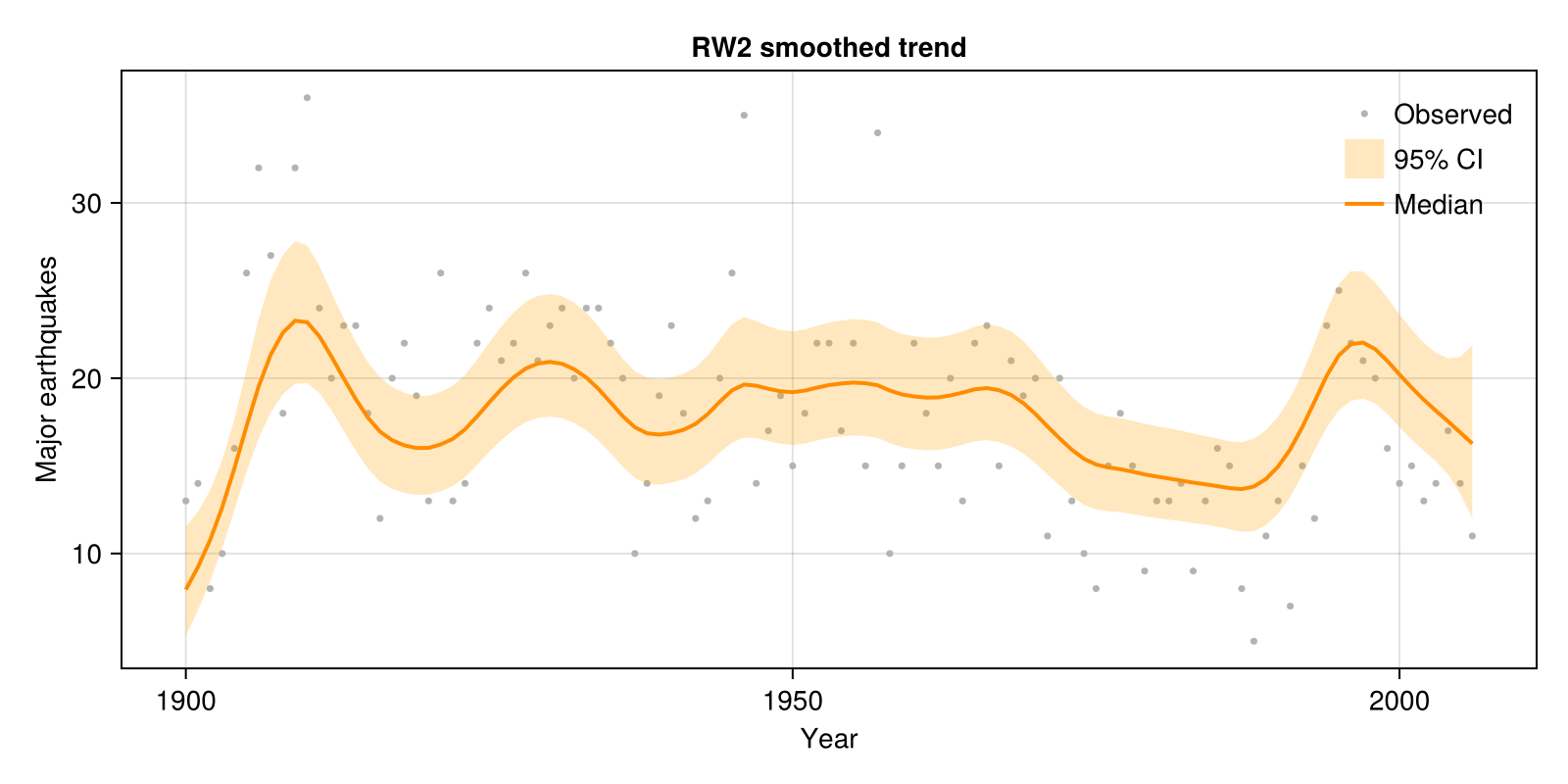

The RW2 trend is noticeably smoother. Instead of tracking year-to-year noise, it captures the broad shape: a rise from 1900 to the 1940s, a gradual plateau, and a decline from the 1970s onwards.

Side-by-side comparison

The contrast between RW1 and RW2 shows how the smoothness assumption feeds through to the fitted trend. Let's overlay both:

julia

fig = Figure(size = (900, 450))
ax = Axis(
    fig[1, 1],
    xlabel = "Year", ylabel = "Major earthquakes",
    title = "RW1 vs RW2: the effect of smoothness assumptions"
)
scatter!(ax, eq_data.year, eq_data.quakes, color = :gray70, markersize = 5, label = "Observed")
lines!(ax, fit_rw1.year, fit_rw1.median, color = :steelblue, linewidth = 2, label = "RW1 (first-order)")
lines!(ax, fit_rw2.year, fit_rw2.median, color = :darkorange, linewidth = 2, label = "RW2 (second-order)")
axislegend(ax, position = :rt, framevisible = false)
fig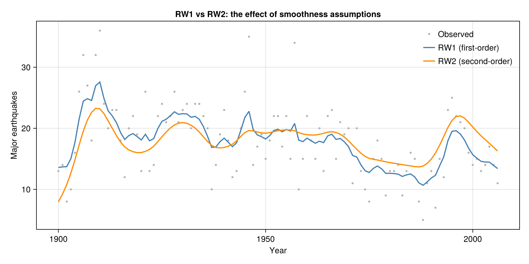

The RW1 trend (blue) hugs the data more closely, while the RW2 trend (orange) is smoother and tells a simpler story about the underlying process. Neither is "right" in an absolute sense; the choice depends on whether you believe the true rate changes erratically or smoothly.

Hyperparameter posteriors

The precision $τ$ controls the bias-variance tradeoff. Let's examine its posterior for each model:

julia

fig = Figure(size = (900, 400))
ax1 = Axis(
    fig[1, 1],
    xlabel = "Precision (τ)", ylabel = "Density",
    title = "RW1 precision posterior"
)
ax2 = Axis(
    fig[1, 2],
    xlabel = "Precision (τ)", ylabel = "Density",
    title = "RW2 precision posterior"
)
plot!(ax1, hyperparameter_marginals(result_rw1, :τ_rw)[1])
plot!(ax2, hyperparameter_marginals(result_rw2, :τ_rw)[1])
fig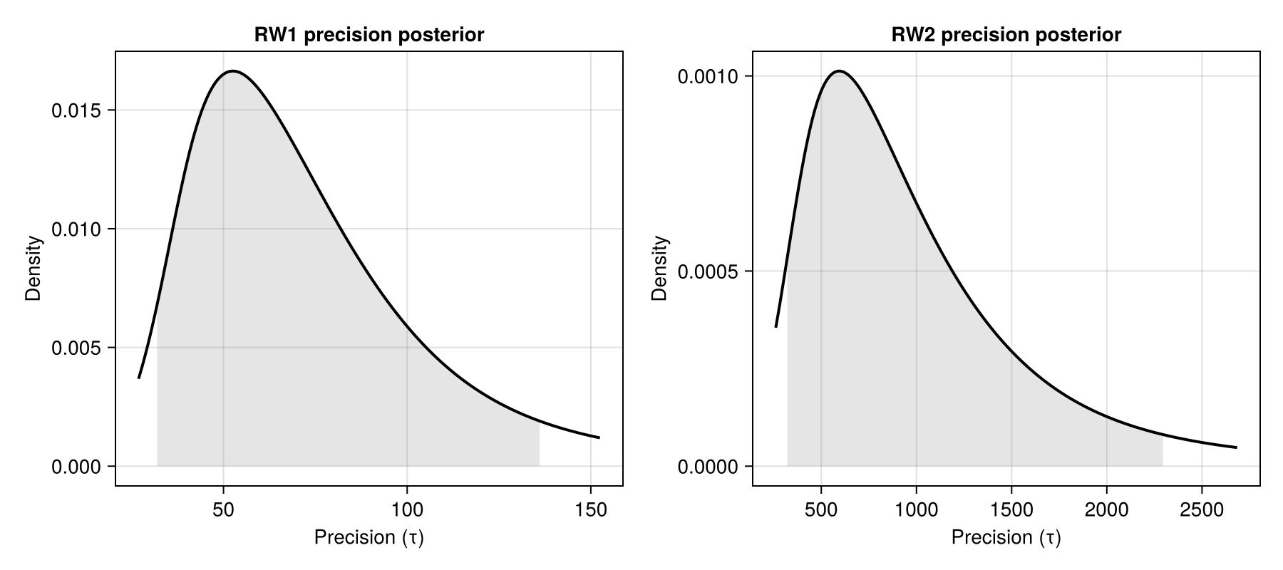

Higher precision means smaller differences between consecutive time points, which produces a smoother curve. The two posteriors sit in different places: the data inform how much smoothing is appropriate within each model class.

The posterior mean of $τ$ is read directly off the marginal, since @latte reports hyperparameters on their declared (natural) scale:

julia

τ_rw1 = hyperparameter_marginals(result_rw1, :τ_rw)[1]
τ_rw2 = hyperparameter_marginals(result_rw2, :τ_rw)[1]
mean(τ_rw1), mean(τ_rw2)

(70.47269658135141, 1010.3205803250598)

A compact summary table for each model's precision:

julia

summary_df(hyperparameter_marginals(result_rw1))

1×6 DataFrame
 Row │ mode     median   q2_5     q97_5    mean     std
     │ Float64  Float64  Float64  Float64  Float64  Float64
─────┼──────────────────────────────────────────────────────
   1 │ 52.5635  65.1534  31.6127  136.505  70.4727  27.3263

julia

summary_df(hyperparameter_marginals(result_rw2))

1×6 DataFrame
 Row │ mode     median   q2_5     q97_5    mean     std
     │ Float64  Float64  Float64  Float64  Float64  Float64
─────┼──────────────────────────────────────────────────────
   1 │ 597.223  858.423  309.985  2595.94  1010.32   583.56

Model comparison

Which model fits the data better? INLA computes several model comparison criteria as part of inference, and they land in result.accumulators. We pull out three. The Deviance Information Criterion (DIC) and the Watanabe-Akaike Information Criterion (WAIC) both balance fit against complexity, with lower values preferred; the log marginal likelihood is a model-selection score where higher is preferred. The default accumulator tuple orders them as DIC, log marginal likelihood, then WAIC.

julia

comparison = DataFrame(
    model = String[], DIC = Float64[], p_D = Float64[],
    WAIC = Float64[], log_ML = Float64[],
)
for (name, res) in [("RW1", result_rw1), ("RW2", result_rw2)]
    push!(
        comparison, (
            name,
            round(res.accumulators[1].DIC, digits = 1),
            round(res.accumulators[1].p_D, digits = 1),
            round(res.accumulators[3].WAIC, digits = 1),
            round(res.accumulators[2].log_marginal_likelihood, digits = 1),
        )
    )
end
comparison

2×5 DataFrame
 Row │ model   DIC      p_D      WAIC     log_ML
     │ String  Float64  Float64  Float64  Float64
─────┼────────────────────────────────────────────
   1 │ RW1       586.9      1.0    634.5   -338.9
   2 │ RW2       646.1      0.7    679.7   -358.8

DIC and WAIC weigh fit against complexity. The effective number of parameters ( $p_{D}$ ) is lower for RW2, reflecting its smoother fit, so the criteria let us ask whether the extra flexibility of RW1 earns its keep on this data.

Posterior predictive check

Finally, do the models reproduce the variability we see in the data? We draw posterior predictive datasets with posterior_predictive, which returns an n_samples × n_obs matrix where each row is one simulated dataset:

julia

using Random
Random.seed!(42)

n_obs = nrow(eq_data)
n_samples = 200
pp_rw1 = posterior_predictive(result_rw1, n_samples)
pp_rw2 = posterior_predictive(result_rw2, n_samples)
size(pp_rw1), size(pp_rw2)

((200, 107), (200, 107))

For each year, take the 2.5th and 97.5th percentiles over the replicated counts (columns index years here):

julia

pp_rw1_lo = [quantile(pp_rw1[:, t], 0.025) for t in 1:n_obs]
pp_rw1_hi = [quantile(pp_rw1[:, t], 0.975) for t in 1:n_obs]
pp_rw2_lo = [quantile(pp_rw2[:, t], 0.025) for t in 1:n_obs]
pp_rw2_hi = [quantile(pp_rw2[:, t], 0.975) for t in 1:n_obs];

fig = Figure(size = (900, 500))
ax1 = Axis(
    fig[1, 1], xlabel = "Year", ylabel = "Count",
    title = "Posterior predictive: RW1"
)
ax2 = Axis(
    fig[1, 2], xlabel = "Year", ylabel = "Count",
    title = "Posterior predictive: RW2"
)
band!(ax1, eq_data.year, pp_rw1_lo, pp_rw1_hi, color = (:steelblue, 0.2))
scatter!(ax1, eq_data.year, eq_data.quakes, color = :gray40, markersize = 4)
band!(ax2, eq_data.year, pp_rw2_lo, pp_rw2_hi, color = (:orange, 0.2))
scatter!(ax2, eq_data.year, eq_data.quakes, color = :gray40, markersize = 4)
fig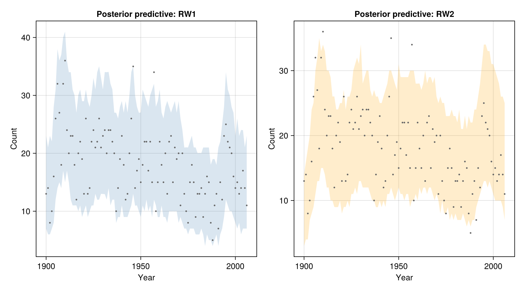

The shaded bands show where 95% of replicated data would fall. If the observed counts sit comfortably inside the bands, the model is capturing the data's variability well. Points consistently outside the bands would suggest model misspecification.

Summary

We used INLA to smooth earthquake counts over a century of data, with a few points worth carrying forward:

RW1 penalises first differences and gives a locally adaptive trend that can change direction easily, which suits a process you expect to move irregularly.
RW2 penalises second differences for a globally smooth trend, a better match when the underlying rate varies slowly.
Within each model class the precision $τ$ sets the degree of smoothing, and INLA estimates it from the data rather than leaving it for you to pick.
DIC, WAIC, and the marginal likelihood give principled ways to compare models with different smoothness assumptions.

Random walks are basic building blocks in INLA (Rue & Held, 2005). From RW1 and RW2 you can build toward AR1 processes, seasonal models, and the separable space-time models covered in the spatial disease mapping tutorial.