
Earthquake Intensity: Spatial Modelling with the SPDE Approach
The SPDE approach (Lindgren, Rue & Lindström, 2011) represents a continuously indexed spatial random field as a Gaussian Markov random field on a triangular mesh. That gives the modelling flexibility of a geostatistical Matérn field while keeping the sparse precision matrices that make inference tractable.
Here we fit a log-Gaussian Cox process to earthquake data. Given the locations of M ≥ 4.5 earthquakes around Japan in 2023, we estimate the underlying seismic intensity surface, and the fitted Matérn field recovers the plate boundary geometry (the Japan Trench, the Izu-Bonin arc, the Kuril arc) from the counts alone.
Along the way the tutorial covers:
downloading and gridding a spatial point pattern into Poisson counts,
why a Poisson observation model over a Matérn field is a log-Gaussian Cox process,
evaluating the fitted field at new locations with
linear_combinations, andoverlaying the result on a coastline map.
Downloading earthquake data
We query the USGS Earthquake Catalog for all M ≥ 4.5 earthquakes in the Japan region during 2023. The API returns a CSV that we read directly into a DataFrame.
using Downloads, CSV, DataFrames

usgs_url = "https://earthquake.usgs.gov/fdsnws/event/1/query?" *
    "format=csv&starttime=2023-01-01&endtime=2024-01-01&minmagnitude=4.5" *
    "&minlatitude=25&maxlatitude=50&minlongitude=125&maxlongitude=150"
eq = CSV.read(Downloads.download(usgs_url), DataFrame)
nrow(eq)587Binning into a spatial grid
A log-Gaussian Cox process models the intensity (expected events per unit area) as a function of space. To turn point locations into observations for INLA, we lay down a regular grid and count events per cell. Each cell becomes one Poisson observation with the cell area as exposure:
where
n_grid = 15
lat_range = (25.0, 50.0)
lon_range = (125.0, 150.0)
dlat = (lat_range[2] - lat_range[1]) / n_grid
dlon = (lon_range[2] - lon_range[1]) / n_grid

grid_lats = [lat_range[1] + (i - 0.5) * dlat for i in 1:n_grid]
grid_lons = [lon_range[1] + (j - 0.5) * dlon for j in 1:n_grid]

cell_counts = zeros(Int, n_grid, n_grid)
for row in eachrow(eq)
    i = clamp(ceil(Int, (row.latitude - lat_range[1]) / dlat), 1, n_grid)
    j = clamp(ceil(Int, (row.longitude - lon_range[1]) / dlon), 1, n_grid)
    cell_counts[i, j] += 1
end

df = DataFrame(
    lat = vec([lat for lat in grid_lats, _ in grid_lons]),
    lon = vec([lon for _ in grid_lats, lon in grid_lons]),
    count = vec(cell_counts),
    area = fill(dlat * dlon, n_grid^2),
)
first(df, 5)
5×4 DataFrame
Row │ lat lon count area
│ Float64 Float64 Int64 Float64
─────┼──────────────────────────────────
1 │ 25.8333 125.833 14 2.77778
2 │ 27.5 125.833 0 2.77778
3 │ 29.1667 125.833 0 2.77778
4 │ 30.8333 125.833 0 2.77778
5 │ 32.5 125.833 0 2.77778Let's visualise the raw counts on the grid:
using AlgebraOfGraphics, CairoMakie

# Raw Makie: a geographic heatmap with an epicentre-scatter overlay and a
# colorbar — a layered spatial-field figure AoG does not express cleanly.
fig = Figure(size = (600, 500))
ax = Axis(
    fig[1, 1]; title = "Earthquake counts per grid cell",
    xlabel = "Longitude", ylabel = "Latitude", aspect = DataAspect()
)
hm = heatmap!(ax, grid_lons, grid_lats, cell_counts'; colormap = :YlOrRd)
scatter!(ax, eq.longitude, eq.latitude; color = :black, markersize = 2)
Colorbar(fig[1, 2], hm; label = "Count")
fig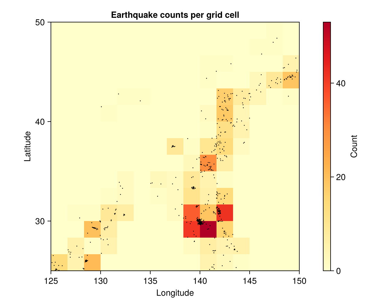
The earthquakes cluster along narrow bands, the subduction zones where tectonic plates collide; most of the domain has zero or very few events. A spatial field is a natural way to capture this structure while sharing information across cells.
Building the Matérn mesh
The SPDE approach discretises the Matérn field on a triangular finite-element mesh. MaternModel(points; smoothness = 1) builds the mesh from a set of observation points (via their convex hull) and stores a projection matrix A_obs from mesh degrees of freedom to those points. At inference time the latent field lives on the mesh DOFs; at each observation, the linear predictor reads field through the projection.
using GaussianMarkovRandomFieldsActivate the GaussianMarkovRandomFields FEM extension: MaternModel builds an SPDE / finite-element representation, so it needs Ferrite + FerriteGmsh + Gmsh (plus LibGEOS to derive the mesh domain from the observation hull).
using Ferrite, FerriteGmsh, Gmsh, LibGEOS

obs_points = hcat(df.lon, df.lat)   # N × 2 — lon first, then lat
base_matern = MaternModel(obs_points; smoothness = 1)
A_obs = evaluation_matrix(base_matern)
n_mesh = length(base_matern)

println("Mesh DOFs: ", n_mesh)
println("A_obs size: ", size(A_obs))
Mesh DOFs: 581
A_obs size: (225, 581)The model
The Matérn field has two hyperparameters: the field precision τ_matern (controlling amplitude) and range_matern (controlling spatial correlation distance). We use a PC prior for precision and an Exponential prior for range.
using Latte
using Distributions
using LinearAlgebra

@latte function spde_model(counts, area, base_matern, A_obs)
    τ_matern ~ PCPrior.Precision(1.0, α = 0.01)
    range_matern ~ Exponential(5.0)
    β ~ MvNormal(zeros(1), 100.0 * I(1))
    field ~ base_matern(τ = τ_matern, range = range_matern)
    η = β[1] .+ A_obs * field
    for i in eachindex(counts)
        counts[i] ~ Poisson(area[i] * exp(η[i]))
    end
end
spde_model (generic function with 1 method)Running INLA
We hand the model and the counts to inla. With no marginalization method specified, Latte picks its default for this kind of model, which corrects the Gaussian-approximation mean of the latent field. That correction matters for count data, where the posterior can be skewed at cells with few or zero events.
lgm = spde_model(df.count, df.area, base_matern, A_obs)
result = inla(lgm, df.count; progress = false)
INLAResult:
Model: LatentGaussianModel{HyperparameterSpec{@NamedTuple{τ_matern::Hyperparameter{Bijectors.TruncatedBijector{Float64, Float64}, :natural}, range_matern::Hyperparameter{Base.Fix1{typeof(broadcast), typeof(log)}, :natural}}, @NamedTuple{}}, Latte._PatternAugmentedLatentModel{Latte.RoutedLatentModel{CombinedModel{LinearSolve.CHOLMODFactorization{Nothing}}, @NamedTuple{τ_matern::Symbol, range_matern::Symbol}}, SparseArrays.SparseMatrixCSC{Int64, Int64}}, LinearlyTransformedObservationModel{ExponentialFamily{Distributions.Poisson, LogLink, Nothing, Nothing}, SparseArrays.SparseMatrixCSC{Float64, Int64}, Vector{Float64}}}
Hyperparameters: 2
Latent variables: 582
Mode: (τ_matern=0.1641, range_matern=5.9455)
Convergence: ✓
Total time: 13.39 seconds
Exploration: 17 points (17 integration)
Model comparison metrics:
Deviance Information Criterion (DIC):
DIC: 294.97
Effective parameters (p_D): -0.08
Mean deviance (D̄): 295.05
Deviance at mode: 295.13
Marginal Log-Likelihood:
log p(y): -308.41
Watanabe-Akaike Information Criterion (WAIC):
WAIC: 447.2
Effective parameters (p_WAIC): 48.27
Log pointwise predictive density (lppd): -175.33
Conditional Predictive Ordinates (CPO):
LPML: -2.92832824e6
Mean CPO: 0.0
Min CPO: 0.0
Unreliable observations: 225 / 225
Max failure score: 173.56
PIT computed: 225 values
PIT mean: 0.4573 (ideal: 0.5)
Approximation quality (KLD):
Max SKLD: 1.7867 (variable 1)
Mean SKLD: 0.3615
Use .hyperparameter_marginals, .latent_marginals, .accumulators for analysisHyperparameter posteriors
A compact table of what the model learned about the spatial structure. Both hyperparameters are reported on their natural declared scale.
summary_df(hyperparameter_marginals(result))2×6 DataFrame
Row │ mode median q2_5 q97_5 mean std
│ Float64 Float64 Float64 Float64 Float64 Float64
─────┼────────────────────────────────────────────────────────────
1 │ 0.15269 0.161831 0.104288 0.248819 0.165676 0.0376865
2 │ 5.86636 5.95558 4.85656 7.31363 5.9911 0.637805The estimated spatial range is the characteristic scale of seismic intensity variation: roughly how far the influence of a plate boundary reaches.
hyper_df = mapreduce(
    vcat, [
        (:τ_matern, "Field precision τ"), (:range_matern, "Spatial range (degrees)"),
    ]
) do (name, label)
    d = hyperparameter_marginals(result, name)[1]
    μ, s = mean(d), std(d)
    xs = range(max(1.0e-3, μ - 4s), μ + 4s; length = 200)
    DataFrame(parameter = label, value = xs, density = pdf.(d, xs))
end

data(hyper_df) *
    mapping(:value => "value", :density => "density", layout = :parameter) *
    visual(Lines, color = :steelblue, linewidth = 2) |>
    x -> draw(x; facet = (; linkxaxes = :none, linkyaxes = :none))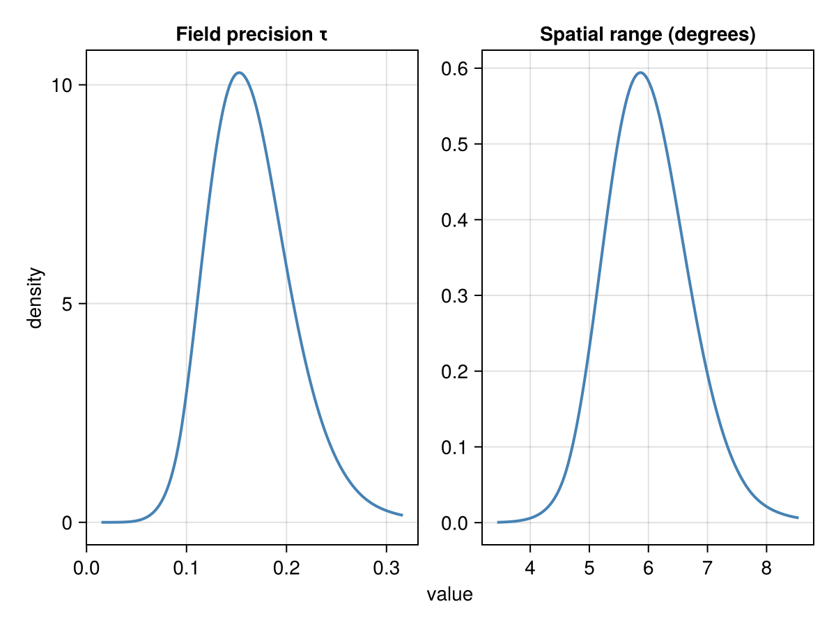
Predicting the intensity surface
To evaluate the fitted Matérn field on a fine prediction grid, we build a projection matrix A_pred from the same FEM discretization to the new locations and ask for the marginal of β + A_pred_row · field at each prediction point. linear_combinations(result; β = 1.0, field = A_pred) does the bookkeeping: each keyword names a latent block and gives its coefficients, and any block left out is treated as a zero column.
n_fine = 50
fine_lats = range(lat_range[1], lat_range[2]; length = n_fine)
fine_lons = range(lon_range[1], lon_range[2]; length = n_fine)

pred_points = hcat(
    vec([lon for _ in fine_lats, lon in fine_lons]),
    vec([lat for lat in fine_lats, _ in fine_lons]),
)
A_pred = evaluation_matrix(base_matern.discretization, pred_points)

pred_marginals = linear_combinations(result; β = 1.0, field = A_pred)
length(pred_marginals), mean(first(pred_marginals))   # one marginal per grid point
(2500, -0.08073228930734574)The named latent blocks are also addressable on their own. The accessor functions work whether or not Latte materializes the linear predictor, so reaching for the intercept is just latent_marginals(result, :β):
summary_df(latent_marginals(result, :β))1×6 DataFrame
Row │ mode median q2_5 q97_5 mean std
│ Float64 Float64 Float64 Float64 Float64 Float64
─────┼────────────────────────────────────────────────────────────
1 │ -3.66542 -3.78271 -5.61339 -2.40927 -3.84286 0.813041The predictions are on the linear predictor scale (log-intensity). We exponentiate to get the intensity itself (expected events per degree²).
pred_means = mean.(pred_marginals)
intensity = reshape(exp.(pred_means), n_fine, n_fine)'
size(intensity)
(50, 50)Visualising the intensity surface
We overlay the predicted intensity on a coastline map to see how the model's spatial structure aligns with real tectonic features. The coastline data comes from Natural Earth (public domain, ~137 KB).
coast_url = "https://raw.githubusercontent.com/nvkelso/natural-earth-vector/" *
    "master/geojson/ne_110m_coastline.geojson"
coast_str = read(Downloads.download(coast_url), String);

function extract_coastline_segments(geojson_str, lon_range, lat_range)
    segments = Vector{Tuple{Vector{Float64}, Vector{Float64}}}()
    for m in eachmatch(r"\[\[[-\d.]+,[-\d.]+\](?:,\[[-\d.]+,[-\d.]+\])*\]", geojson_str)
        lons, lats = Float64[], Float64[]
        for coord in eachmatch(r"\[([-\d.]+),([-\d.]+)\]", m.match)
            lon = parse(Float64, coord.captures[1])
            lat = parse(Float64, coord.captures[2])
            if lon_range[1] - 5 <= lon <= lon_range[2] + 5 &&
                    lat_range[1] - 5 <= lat <= lat_range[2] + 5
                push!(lons, lon)
                push!(lats, lat)
            else
                length(lons) > 1 && push!(segments, (copy(lons), copy(lats)))
                empty!(lons); empty!(lats)
            end
        end
        length(lons) > 1 && push!(segments, (copy(lons), copy(lats)))
    end
    return segments
end
coastlines = extract_coastline_segments(coast_str, lon_range, lat_range)
length(coastlines)   # number of coastline segments in the window

# Raw Makie: the predicted field on the FEM grid with a log-scaled colorbar,
# coastline lines, and an epicentre scatter overlaid — a spatial composite
# outside AoG's data-mapping idiom.
fig = Figure(size = (700, 600))
ax = Axis(
    fig[1, 1]; title = "Predicted seismic intensity — Japan, 2023 (M ≥ 4.5)",
    xlabel = "Longitude", ylabel = "Latitude", aspect = DataAspect()
)
hm = heatmap!(
    ax, collect(fine_lons), collect(fine_lats), intensity;
    colormap = :inferno, colorscale = log10
)
for (lons, lats) in coastlines
    lines!(ax, lons, lats; color = :white, linewidth = 1.5)
end
scatter!(
    ax, eq.longitude, eq.latitude;
    color = :cyan, markersize = 3, strokewidth = 0.5, strokecolor = :black
)
xlims!(ax, lon_range...)
ylims!(ax, lat_range...)
Colorbar(fig[1, 2], hm; label = "Events per deg²")
fig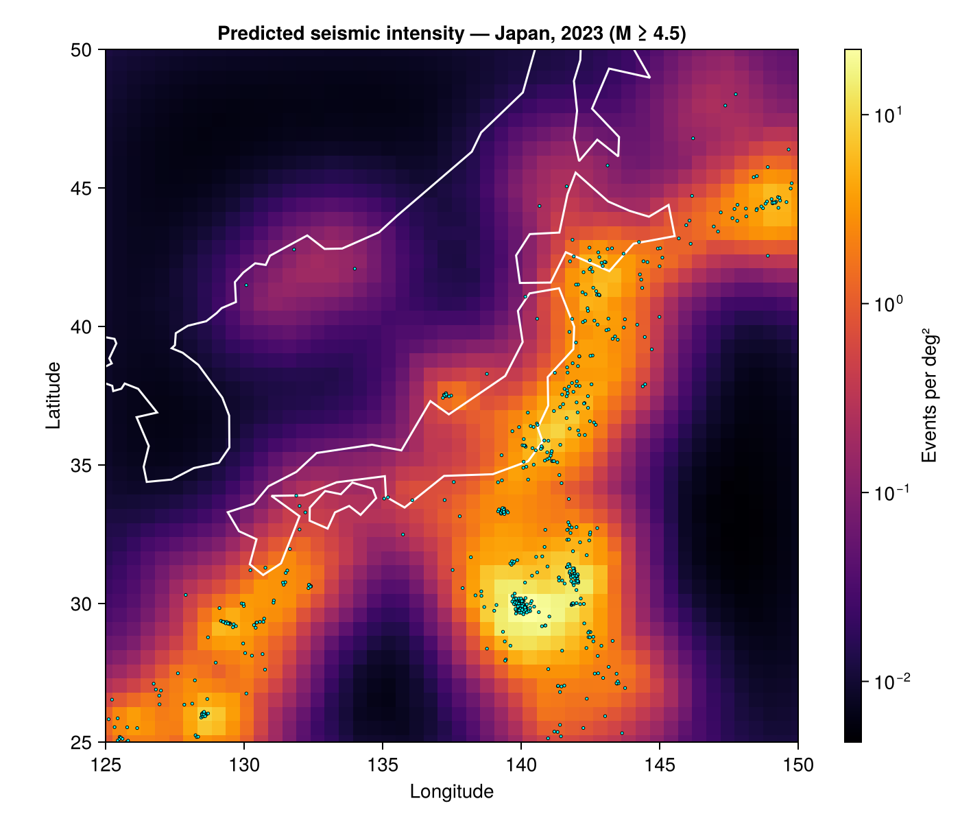
The fitted surface lines up with the major tectonic features, recovered from the counts alone:
the Japan Trench (140–145°E, 35–43°N), the main subduction zone where the Pacific Plate dives under northeastern Japan;
the Izu-Bonin arc (~140°E, 28–33°N), an active volcanic arc running south from Tokyo;
the Kuril arc (~148°E, 44°N), the northern continuation of the subduction zone;
the Ryukyu arc (~126–128°E, 25–30°N), the southwestern island chain;
the Sea of Japan interior, picked out as a low-intensity region.
The Matérn field interpolates between the observed grid cells, sharing spatial information to estimate intensity even where no earthquakes were recorded.
Posterior uncertainty
The fit returns full posterior marginals, not just point estimates, so we can map the posterior standard deviation of the field alongside its mean:
pred_sds = std.(pred_marginals)
sd_grid = reshape(pred_sds, n_fine, n_fine)';

# Raw Makie: same spatial-field-plus-coastline composite as above, here for
# the posterior SD grid.
fig = Figure(size = (700, 600))
ax = Axis(
    fig[1, 1]; title = "Posterior uncertainty (std. dev. of log-intensity)",
    xlabel = "Longitude", ylabel = "Latitude", aspect = DataAspect()
)
hm = heatmap!(ax, collect(fine_lons), collect(fine_lats), sd_grid; colormap = :YlOrRd)
for (lons, lats) in coastlines
    lines!(ax, lons, lats; color = :black, linewidth = 1)
end
xlims!(ax, lon_range...)
ylims!(ax, lat_range...)
Colorbar(fig[1, 2], hm; label = "Posterior SD")
fig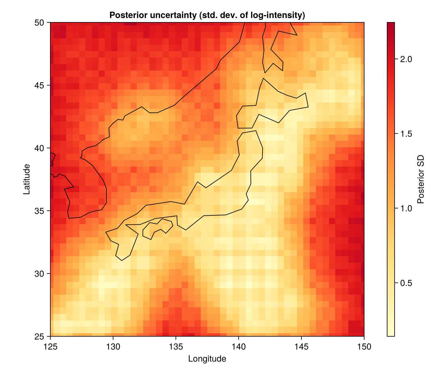
Uncertainty is lowest in areas with many observations (the active subduction zones) and highest in data-sparse regions (open ocean, continental interior).
Model diagnostics
The default accumulators report DIC and WAIC for model comparison, and log_marginal_likelihood returns the grid estimate of log p(y).
println("Model fit:")
println("  DIC:  $(round(result.accumulators[1].DIC, digits = 1))")
println("  WAIC: $(round(result.accumulators[3].WAIC, digits = 1))")
println("  Log marginal likelihood: $(round(log_marginal_likelihood(result), digits = 1))")
Model fit:
DIC: 295.0
WAIC: 447.2
Log marginal likelihood: -308.4Summary
We fit a log-Gaussian Cox process to earthquake data with INLA and the SPDE approach. From the gridded epicentre counts we estimated a continuous seismic intensity surface that recovers the geometry of the major plate boundaries, with no geological prior knowledge.
A few points worth carrying over to other spatial models:
MaternModel(points; smoothness = ν)builds the FEM mesh, the SPDE discretisation, and the projection matrix in one step, andevaluation_matrixis the reusable design-matrix operator for new locations.A Poisson likelihood with an exposure term turns gridded counts into a log-Gaussian Cox process; the exposure enters as a log-offset in the linear predictor.
linear_combinations(result; β = 1.0, field = A_pred)evaluates the fitted field at arbitrary locations, with each keyword naming a latent block and supplying its coefficients.Because the fit returns full marginals, the same machinery gives posterior uncertainty on the intensity surface and on the hyperparameters.
Data sources: the USGS Earthquake Hazards Program (epicentre catalogue) and Natural Earth (public-domain coastlines).
References
The SPDE approach: representing a continuously indexed Matérn field as a Gaussian Markov random field on a triangular mesh, giving geostatistical flexibility with sparse precision matrices.
Penalised-complexity priors for the range and marginal variance of a Matérn field, the interpretable joint prior used here for the SPDE hyperparameters.
This page was generated using Literate.jl.