
When to sample the hyperparameters: HMC-Laplace vs INLA
INLA gains its speed from a deliberate shortcut. The latent field is integrated out with a Laplace (Gaussian) approximation, and the hyperparameters are integrated out over a small, fixed set of design points: a grid for one or two hyperparameters, a Central Composite Design (CCD) for three or more. That design sits on an ellipsoid scaled by the curvature (Hessian) of the posterior at its mode.
The approximation is good when the hyperparameter posterior is roughly Gaussian in the transformed (working) space, which is usually the case, and then INLA is both fast and accurate. The assumption can fail, though. When the hyperparameter posterior is a curved, skewed ridge, a symmetric ellipsoidal design cannot follow the curve, and the resulting marginals are biased, typically by truncating the skewed tails.
hmc_laplace keeps the inner Laplace approximation for the latent field and replaces the deterministic hyperparameter design with NUTS (Hoffman & Gelman, 2014), sampling the hyperparameter posterior directly. This embedded-Laplace-within-HMC scheme follows Margossian et al. (2020). It costs more than INLA, though much less than full MCMC since the latent field is still integrated out analytically, and in return it tracks whatever shape the hyperparameter posterior actually has.
This tutorial builds a model whose hyperparameter posterior is genuinely non-Gaussian, shows that INLA-CCD is biased there, checks HMC-Laplace against a validated gold-standard MCMC reference, and closes with a guide to choosing between the two.
A model with a curved hyperparameter posterior
An AR(1) latent process manufactures this geometry cleanly. It has two hyperparameters that trade off against each other: the innovation precision τ_ar (inverse variance), and the lag-1 correlation ρ, with 0 < ρ < 1.
On short or noisy series the data constrain the overall smoothness of the path well, but not the split between "high precision, high correlation" and "low precision, low correlation". The result is a curved ridge in (τ_ar, ρ) space, made worse by ρ piling up against its upper boundary at
- Adding an IID observation-level effect (a third hyperparameter
τ_iid)
pushes INLA onto its CCD design rather than a dense grid, and CCD is where the ellipsoidal-design assumption bites.
using Latte
using Distributions
using GaussianMarkovRandomFields: AR1Model, IIDModel
using Turing
using LinearAlgebra
using Random, Statistics, Printf
using DataFrames
using CairoMakie
The @latte model below is what inla and hmc_laplace consume. The PC prior on ρ shrinks toward the base model ρ = 0, and the PC priors on the precisions shrink toward infinite precision (zero variance).
@latte function ar1_counts(y, n)
    τ_ar ~ PCPrior.Precision(1.0, α = 0.01)
    ρ ~ PCPrior.AR1Correlation(0.7; α = 0.1, positive_only = true)
    τ_iid ~ PCPrior.Precision(1.0, α = 0.01)
    f ~ AR1Model(n)(τ = τ_ar, ρ = ρ)
    u ~ IIDModel(n)(τ = τ_iid)
    for i in eachindex(y)
        y[i] ~ Poisson(exp(f[i] + u[i]); check_args = false)
    end
end
ar1_counts (generic function with 1 method)Simulate a moderately persistent series with relatively few counts, so the hyperparameter posterior is genuinely uncertain.
Random.seed!(20260606)
n = 40
ρ_true, σ_ar = 0.88, 0.5
f_true = zeros(n)
f_true[1] = randn() * σ_ar / sqrt(1 - ρ_true^2)
for i in 2:n
    f_true[i] = ρ_true * f_true[i - 1] + randn() * σ_ar
end
η = f_true .+ randn(n) * 0.2 .- mean(f_true) .+ 1.0
y = rand.(Poisson.(exp.(η)))
@printf("simulated %d time points, total count %d, max %d\n", n, sum(y), maximum(y))

lgm = ar1_counts(y, n)
LatentGaussianModel
├─ hyperparameters (3)
│ τ_ar ~ PCPrior.Precision(λ=4.605)
│ ρ ~ PCPrior.AR1Correlation(λ=2.806, positive_only=true)
│ τ_iid ~ PCPrior.Precision(λ=4.605)
├─ latent field · 80 dims
│ f 40 AR
│ u 40 IID
└─ likelihood
Poisson, log link · 40 observationsTwo ways to integrate out the hyperparameters
Same model object, two engines. inla uses the deterministic CCD design; hmc_laplace samples the hyperparameters with NUTS, warm-started from the Laplace approximation at the mode.
hp = (:τ_ar, :ρ, :τ_iid)(:τ_ar, :ρ, :τ_iid)A warm-up pass compiles both engines, so the runtimes below time the inference rather than first-call compilation.
inla(lgm, y; progress = false)
hmc_laplace(lgm, y; n_samples = 10, n_warmup = 10, diff_strategy = FiniteDiffStrategy(), rng = MersenneTwister(0));

t_inla = @elapsed result_inla = inla(lgm, y; progress = false)
t_hmc = @elapsed result_hmc = hmc_laplace(
    lgm, y; n_samples = 2000, n_warmup = 1000,
    diff_strategy = FiniteDiffStrategy(), rng = MersenneTwister(1),
)
@printf("INLA used %d CCD design points\n", length(result_inla.exploration.grid_points))
@printf("HMC-Laplace: converged=%s, divergences=%d\n", converged(result_hmc), divergences(result_hmc))
@printf("runtime — INLA: %.2f s     HMC-Laplace: %.1f s   (≈%.0f× INLA)\n", t_inla, t_hmc, t_hmc / t_inla)
┌ Info: Finished 10 adaptation steps
│ adaptor =
│ NesterovDualAveraging{Float64} with
│ Scaling γ=0.05
│ Starting iter t_0=10.0
│ Shrinkage κ=0.75
│ Target statistic δ=0.8
│ Current ϵ=0.4616791476279187
│ κ.τ.integrator = Leapfrog with step size ϵ=0.462
│ h.metric =
│ DenseEuclideanMetric{Float64} with size (3,) mass matrix:
└ [0.317751, 0.591505, 3.3358 ...]
┌ Info: Finished 10 sampling steps for 1 chains in 0.241951701 (s)
│ h = Hamiltonian with DenseEuclideanMetric and GaussianKinetic
│ κ = AdvancedHMC.HMCKernel{AdvancedHMC.FullMomentumRefreshment, AdvancedHMC.Trajectory{AdvancedHMC.MultinomialTS, AdvancedHMC.Leapfrog{Float64}, AdvancedHMC.GeneralisedNoUTurn{Float64}}}(AdvancedHMC.FullMomentumRefreshment(), Trajectory{AdvancedHMC.MultinomialTS} with Leapfrog with step size ϵ=0.462 and termination criterion AdvancedHMC.GeneralisedNoUTurn{Float64}(10, 1000.0))
│ EBFMI_est = 0.844206635738528
└ average_acceptance_rate = 0.6988714587779083
┌ Info: Finished 1000 adaptation steps
│ adaptor =
│ NesterovDualAveraging{Float64} with
│ Scaling γ=0.05
│ Starting iter t_0=10.0
│ Shrinkage κ=0.75
│ Target statistic δ=0.8
│ Current ϵ=0.7638917674863376
│ κ.τ.integrator = Leapfrog with step size ϵ=0.764
│ h.metric =
│ DenseEuclideanMetric{Float64} with size (3,) mass matrix:
└ [0.317751, 0.591505, 3.3358 ...]
┌ Info: Finished 2000 sampling steps for 1 chains in 26.583946733 (s)
│ h = Hamiltonian with DenseEuclideanMetric and GaussianKinetic
│ κ = AdvancedHMC.HMCKernel{AdvancedHMC.FullMomentumRefreshment, AdvancedHMC.Trajectory{AdvancedHMC.MultinomialTS, AdvancedHMC.Leapfrog{Float64}, AdvancedHMC.GeneralisedNoUTurn{Float64}}}(AdvancedHMC.FullMomentumRefreshment(), Trajectory{AdvancedHMC.MultinomialTS} with Leapfrog with step size ϵ=0.764 and termination criterion AdvancedHMC.GeneralisedNoUTurn{Float64}(10, 1000.0))
│ EBFMI_est = 0.9362416979000444
└ average_acceptance_rate = 0.7958435655582266
INLA used 15 CCD design points
HMC-Laplace: converged=true, divergences=5
runtime — INLA: 0.02 s HMC-Laplace: 27.5 s (≈1435× INLA)Both engines expose their hyperparameter posteriors as marginal distribution objects through hyperparameter_marginals(result, name), which returns a one-element vector per name. For INLA each marginal is a spline fit with pdf / cdf / quantile; for HMC-Laplace it is the empirical distribution over the NUTS draws. Either way the same Distributions.jl methods apply, so we read the two posteriors the same way.
inla_marginal(nm) = only(hyperparameter_marginals(result_inla, nm))
hmc_marginal(nm) = only(hyperparameter_marginals(result_hmc, nm))
hmc_marginal (generic function with 1 method)The HMC draws themselves are also useful later for plotting and for the Kolmogorov–Smirnov comparison, so we pull them out of the chain once.
hmc_chain = chain(result_hmc)
hmc_draws = Dict(nm => vec(hmc_chain[nm].data) for nm in hp);
The two already disagree on the correlation ρ, most visibly in the upper tail, which says how persistent the process could plausibly be:
for nm in hp
    mi, mh = inla_marginal(nm), hmc_marginal(nm)
    @printf(
        "%-6s  INLA median=%7.3g (q97.5=%8.3g)   HMC median=%7.3g (q97.5=%8.3g)\n",
        nm, median(mi), quantile(mi, 0.975),
        median(mh), quantile(mh, 0.975),
    )
end
τ_ar INLA median= 2.71 (q97.5= 6.26) HMC median= 3.18 (q97.5= 19.8)
ρ INLA median= 0.77 (q97.5= 0.918) HMC median= 0.81 (q97.5= 0.983)
τ_iid INLA median= 62.6 (q97.5= 804) HMC median= 49.9 (q97.5= 2.5e+04)Who is right? A gold-standard reference
To adjudicate we need the exact hyperparameter posterior, from MCMC. An @latte model is itself a DynamicPPL model, and Latte.dppl_model hands it straight to Turing without rewriting. For this model, though, one sampling subtlety is worth knowing. A centered hierarchical scale, drawing the latent directly at precision τ, gives NUTS a funnel geometry that mixes poorly for a weakly-identified variance component, showing up as low ESS and R̂ > 1. So for a clean reference we write the model in non-centered form (unit-normal innovations scaled by σ = 1/√τ), the same statistical model in a geometry NUTS samples cleanly. INLA and HMC-Laplace need no such care, since they marginalize the latent analytically rather than sampling it.
@model function ar1_gold(y, n)
    τ_ar ~ PCPrior.Precision(1.0, α = 0.01)
    ρ ~ PCPrior.AR1Correlation(0.7; α = 0.1, positive_only = true)
    τ_iid ~ PCPrior.Precision(1.0, α = 0.01)
    σ, σu = 1 / sqrt(τ_ar), 1 / sqrt(τ_iid)
    z ~ filldist(Normal(), n)
    zu ~ filldist(Normal(), n)
    f = Vector{typeof(σ * ρ)}(undef, n)
    f[1] = z[1] * σ / sqrt(1 - ρ^2)
    for i in 2:n
        f[i] = ρ * f[i - 1] + z[i] * σ
    end
    u = zu .* σu
    for i in 1:n
        y[i] ~ Poisson(exp(f[i] + u[i]); check_args = false)
    end
    return (f = f,)
end

gold_model = ar1_gold(y, n)
Random.seed!(7)
gold_chain = sample(gold_model, NUTS(1000, 0.95), MCMCThreads(), 1500, 2; progress = false)
gold_draws = Dict(nm => vec(Array(gold_chain[nm])) for nm in hp);
┌ Warning: Only a single thread available: MCMC chains are not sampled in parallel
└ @ AbstractMCMC ~/.julia/packages/AbstractMCMC/4Fh35/src/sample.jl:544
┌ Info: Found initial step size
└ ϵ = 0.2
┌ Info: Found initial step size
└ ϵ = 0.4Validate the reference before trusting it. We check R̂ and ESS for healthy mixing, and add a coupling check: the sampled innovation scale σ_ar = 1/√τ_ar should track the realized spread of the sampled latent path f. A chain that mixed poorly would show this correlation near zero.
gold_stats = DataFrame(summarystats(gold_chain))
for nm in hp
    idx = findfirst(==(nm), gold_stats.parameters)
    @printf("gold %-6s  R̂=%.3f  ESS=%6.0f\n", nm, gold_stats.rhat[idx], gold_stats.ess_bulk[idx])
end
gold_f = [g.f for g in vec(generated_quantities(gold_model, MCMCChains.get_sections(gold_chain, :parameters)))]
coupling = cor(1 ./ sqrt.(gold_draws[:τ_ar]), [std(fp) for fp in gold_f])
@printf("gold coupling cor(σ_ar, sd(f)) = %.3f\n", coupling)
gold τ_ar R̂=1.001 ESS= 691
gold ρ R̂=1.001 ESS= 856
gold τ_iid R̂=1.002 ESS= 762
gold coupling cor(σ_ar, sd(f)) = 0.841The verdict
With a trustworthy reference we can score both engines. The Kolmogorov–Smirnov distance to the gold measures how far each engine's hyperparameter marginal sits from the truth.
# KS distance to the gold, evaluated at the gold draws. Both engines supply
# a `cdf` on their marginal object: INLA's is the analytic spline, HMC's the
# empirical CDF over its draws.
function ks_to_gold(engine_cdf, gold)
    g = sort(gold)
    m = length(g)
    return maximum(abs(engine_cdf(g[i]) - i / m) for i in 1:m)
end

println("\nKolmogorov–Smirnov distance to the gold standard (smaller is better):")
for nm in hp
    ks_inla = ks_to_gold(x -> cdf(inla_marginal(nm), x), gold_draws[nm])
    ks_hmc = ks_to_gold(x -> cdf(hmc_marginal(nm), x), gold_draws[nm])
    @printf("  %-6s  INLA-CCD = %.3f      HMC-Laplace = %.3f\n", nm, ks_inla, ks_hmc)
end
Kolmogorov–Smirnov distance to the gold standard (smaller is better):
  τ_ar    INLA-CCD = 0.152      HMC-Laplace = 0.027
  ρ       INLA-CCD = 0.165      HMC-Laplace = 0.019
  τ_iid   INLA-CCD = 0.148      HMC-Laplace = 0.028
Across all three hyperparameters HMC-Laplace lands several times closer to the truth. The reason is geometric, and worth seeing directly.
Seeing the banana
Plot the joint posterior of (log τ_ar, ρ). The gold-standard samples trace a curved, skewed ridge: low precision goes with high correlation and vice versa, and the ridge bends. Overlaid are INLA's CCD design points, a small symmetric ellipsoidal cloud centered at the mode. That cloud cannot reach up the curved arm of the ridge toward ρ → 1, which is why INLA truncates the upper tail of ρ (and of the precisions).
ccd_points = [
    convert(NamedTuple, convert(NaturalHyperparameters, p.θ))
        for p in result_inla.exploration.grid_points
];

fig = Figure(size = (760, 340))
ax1 = Axis(
    fig[1, 1], xlabel = "log τ_ar  (innovation precision)", ylabel = "ρ  (correlation)",
    title = "Joint hyperparameter posterior",
)
scatter!(
    ax1, log.(gold_draws[:τ_ar]), gold_draws[:ρ];
    color = (:steelblue, 0.18), markersize = 3, label = "gold (NUTS)"
)
scatter!(
    ax1, [log(p.τ_ar) for p in ccd_points], [p.ρ for p in ccd_points];
    color = :firebrick, markersize = 11, marker = :xcross, label = "INLA CCD design"
)
axislegend(ax1; position = :lt, framevisible = false)Makie.Legend()And the marginal that matters most here, the correlation ρ. INLA's curve falls away too early on the right, while HMC-Laplace matches the gold's reach toward strong persistence.
ax2 = Axis(fig[1, 2], xlabel = "ρ  (correlation)", ylabel = "density", title = "Marginal posterior of ρ")
density!(ax2, gold_draws[:ρ]; color = (:steelblue, 0.25), strokecolor = :steelblue, strokewidth = 2, label = "gold (NUTS)")
density!(ax2, hmc_draws[:ρ]; color = (:seagreen, 0.0), strokecolor = :seagreen, strokewidth = 2, label = "HMC-Laplace")
# INLA's marginal is an analytic spline, not samples, so plot its density directly.
mρ = inla_marginal(:ρ)
ρ_grid = range(quantile(mρ, 1.0e-3), quantile(mρ, 1 - 1.0e-3); length = 400)
lines!(
    ax2, ρ_grid, pdf.(Ref(mρ), ρ_grid);
    color = :firebrick, linewidth = 2, linestyle = :dash, label = "INLA-CCD (spline)"
)
axislegend(ax2; position = :lt, framevisible = false)
fig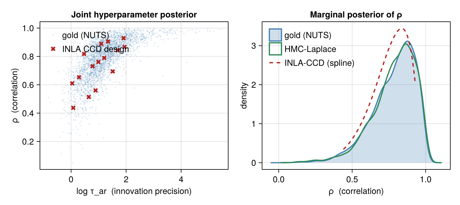
When to reach for HMC-Laplace
INLA is the right default. It is fast, and on most latent Gaussian models the hyperparameter posterior is well-behaved enough that the deterministic design is accurate. Reach past it only when you have a specific reason to.
hmc_laplace earns its extra cost when:
the hyperparameter posterior is curved or strongly skewed, as in scale versus correlation trade-offs (AR and Matérn ranges are the classic cases) or for parameters pinned against a boundary, such as
ρ → 1or a variance heading to zero;you need faithful tails and credible intervals for the hyperparameters themselves, not just their modes, for questions like how persistent the process could plausibly be;
there are only a handful of hyperparameters, so sampling stays affordable.
inla remains the better choice when:
the hyperparameter posterior is roughly Gaussian in the working space (the common case), where CCD is both fast and accurate;
there are many hyperparameters, where MCMC mixing gets hard and the deterministic design scales better;
speed matters and you mainly need posterior means or modes.
A word on cost. HMC-Laplace runs a NUTS chain rather than evaluating a fixed handful of design points, so it is more expensive than INLA. It stays far cheaper than full MCMC on the joint model, though: the latent field, often thousands of dimensions, is integrated out by the inner Laplace approximation at every step, so NUTS only ever explores the low-dimensional hyperparameter space. It is the middle rung between INLA and full HMC, and as here, sometimes the right one.
References
The original INLA paper: deterministic approximate Bayesian inference for latent Gaussian models via nested Laplace approximations and numerical integration over the hyperparameters.
The No-U-Turn Sampler, the adaptive Hamiltonian Monte Carlo algorithm Latte runs over the hyperparameters.
Hamiltonian Monte Carlo over the hyperparameters, with the latent Gaussian field marginalised by an embedded Laplace approximation and the gradient propagated through that inner solve. The method this engine implements.
This page was generated using Literate.jl.