Getting started with Latte.jl

This tutorial walks through a small Bayesian analysis of mortality rates following cardiac surgery across twelve hospitals. We write the model once and then run it through all three of Latte's inference engines, INLA, TMB, and HMC-Laplace, swapping a single function call each time. That "define once, run any engine" workflow is the thread this tutorial pulls on.

Installation

If you haven't done so already, you need to install both Julia and this package:

using Pkg
Pkg.add("Latte")

Latent Gaussian models and the three engines

Latte targets latent Gaussian models (LGMs): hierarchical models with a Gaussian latent field, such as random intercepts, smooth temporal trends, or spatial fields, observed through an exponential-family likelihood. This is a broad class. It covers generalized linear mixed models, geostatistics, and spatio-temporal models built on Gaussian Markov random fields.

For these models the latent field can be integrated out with a Laplace approximation, which is the shared backbone of all three engines Latte ships. They differ only in how they handle the remaining hyperparameters:

• INLA spreads a small grid of hyperparameter points and integrates over them. Deterministic, fast, and the default.

• TMB finds the most likely hyperparameters and fits one Gaussian at that mode. The fastest engine; it reports a mode and standard errors.

• HMC-Laplace samples the hyperparameters with NUTS. The most faithful when the hyperparameter posterior is awkward, and the slowest.

Because they all consume the same LatentGaussianModel, you write the model once and pick the engine afterwards. The rest of this tutorial does exactly that.

The dataset

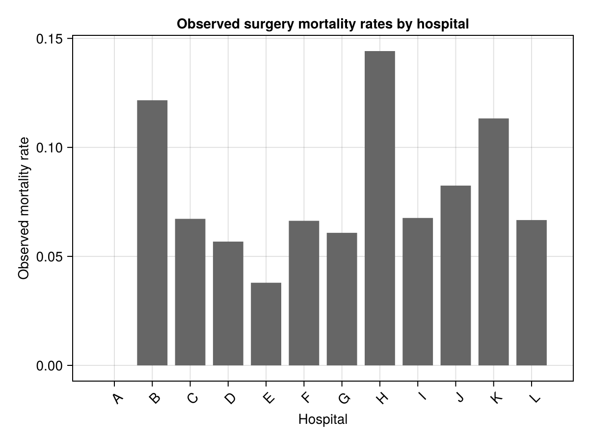
The data records, for each hospital, the number of operations n and the number of deaths r following cardiac surgery on infants. Here it is:

using DataFrames
surg_data = DataFrame(
    hospital = ["A", "B", "C", "D", "E", "F", "G", "H", "I", "J", "K", "L"],
    n = [47, 148, 119, 810, 211, 196, 148, 215, 207, 97, 256, 360],
    r = [0, 18, 8, 46, 8, 13, 9, 31, 14, 8, 29, 24]
)

12×3 DataFrame
 Row │ hospital  n      r
     │ String    Int64  Int64
─────┼────────────────────────
   1 │ A            47      0
   2 │ B           148     18
   3 │ C           119      8
   4 │ D           810     46
   5 │ E           211      8
   6 │ F           196     13
   7 │ G           148      9
   8 │ H           215     31
   9 │ I           207     14
  10 │ J            97      8
  11 │ K           256     29
  12 │ L           360     24

Let's visualize it using AlgebraOfGraphics.jl:

using AlgebraOfGraphics, CairoMakie
draw(
    data(surg_data) *
        mapping(
        :hospital => "Hospital",
        (:r, :n) => ((r, n) -> r ./ n) => "Observed mortality rate"
    ) *
        visual(BarPlot),
    axis = (
        xticklabelrotation = π / 4, title = "Observed surgery mortality rates by hospital",
    )
)

Modelling

Latte.jl models are written as @latte functions, using the same probabilistic programming syntax as DynamicPPL.jl / Turing.jl. If you know Turing, this will look very familiar. @latte recognizes the structured Gaussian priors in the body (here an IIDModel) and builds a LatentGaussianModel that rides Latte's fast inference paths. (Already have a plain Turing @model? The Turing handoff tutorial covers latte_from_dppl.)

For the surgery data, we assume each hospital has its own (logit-scale) mortality rate β + u[h], where β is an overall intercept and u[h] is a hospital-specific random effect with a Gaussian prior. The number of deaths in each hospital is then Binomial.

A few modelling details are worth calling out. The hospital effect u uses IIDModel(H, constraint = :sumtozero)(τ = τ_u), an IID Gaussian random effect whose sum-to-zero constraint keeps β and u identified. The random-effect precision τ_u gets a Gamma(2, 1) prior, which places mild mass on moderate precisions. The inverse-logit link comes from logistic in StatsFuns.

using Latte
using Distributions
using GaussianMarkovRandomFields: IIDModel
using StatsFuns: logistic
using LinearAlgebra

@latte function surg_mortality(r, n_trials, hospital_idx, H)
    τ_u ~ Gamma(2.0, 1.0)
    β ~ MvNormal(zeros(1), 100.0 * I(1))
    u ~ IIDModel(H, constraint = :sumtozero)(τ = τ_u)
    for i in eachindex(r)
        r[i] ~ Binomial(
            n_trials[i], logistic(β[1] + u[hospital_idx[i]])
        )
    end
end

surg_mortality (generic function with 1 method)

Calling the @latte function returns a LatentGaussianModel. Latte reads off which variables form the latent Gaussian field (the "random effects" in mixed-model vocabulary — here β and u) and which are hyperparameters (τ_u) straight from the model body, so there's nothing else to specify.

H = length(surg_data.hospital)
hospital_idx = 1:H |> collect
lgm = surg_mortality(surg_data.r, surg_data.n, hospital_idx, H)

LatentGaussianModel
├─ hyperparameters (1)
│    τ_u  ~ Gamma(α=2.0, θ=1.0)  [log]
├─ latent field · 13 dims
│    β   1   FixedEffects
│    u  12   IID
└─ likelihood
     custom logpdf · 12 observations

Running INLA

With the model in hand, the default engine is one call away:

inla_result = inla(lgm, surg_data.r)

INLAResult:
  Model: LatentGaussianModel{HyperparameterSpec{@NamedTuple{τ_u::Hyperparameter{Base.Fix1{typeof(broadcast), typeof(log)}, :natural}}, @NamedTuple{}}, Latte._PatternAugmentedLatentModel{Latte.RoutedLatentModel{CombinedModel{LinearSolve.CHOLMODFactorization{Nothing}}, @NamedTuple{τ_iid::Symbol}}, SparseArrays.SparseMatrixCSC{Int64, Int64}}, LinearlyTransformedObservationModel{Latte.BinomialTrialsObservationModel{ExponentialFamily{Distributions.Binomial, LogitLink, Nothing, Nothing}, Vector{Int64}}, SparseArrays.SparseMatrixCSC{Float64, Int64}, Nothing}}
  Hyperparameters: 1
  Latent variables: 13
  Mode: (τ_u=3.4264)
  Convergence: ✓
  Total time: 20.01 seconds
  Exploration: 4 points (4 integration)

Model comparison metrics:
Deviance Information Criterion (DIC):
  DIC: 54.26
  Effective parameters (p_D): -0.1
  Mean deviance (D̄): 54.36
  Deviance at mode: 54.47

Marginal Log-Likelihood:
  log p(y): -44.42

Watanabe-Akaike Information Criterion (WAIC):
  WAIC: 67.2
  Effective parameters (p_WAIC): 3.54
  Log pointwise predictive density (lppd): -30.06

Conditional Predictive Ordinates (CPO):
  LPML: -101.09
  Mean CPO: 0.0027
  Min CPO: 0.0
  Unreliable observations: 12 / 12
  Max failure score: 4.52
  PIT computed: 12 values
  PIT mean: 0.4976 (ideal: 0.5)


Approximation quality (KLD):
  Max SKLD: 0.0493 (variable 1)
  Mean SKLD: 0.0057

Use .hyperparameter_marginals, .latent_marginals, .accumulators for analysis

The output is an INLAResult. It holds the full analysis and prints a short summary when displayed.

Every marginal Latte computes implements the Distributions.jl interface, so you can call Distributions.jl methods on these objects directly. The accessor functions return marginals as blocks: one distribution per hyperparameter, one per latent variable. We read them back through these accessors rather than the result's fields, since the accessors behave the same regardless of how the result was stored internally.

For a quick table of key statistics, summary_df collects a block of marginals into a DataFrame. Here are the hyperparameter and latent-field marginals:

summary_df(hyperparameter_marginals(inla_result))

1×6 DataFrame
 Row │ mode     median   q2_5     q97_5    mean     std
     │ Float64  Float64  Float64  Float64  Float64  Float64
─────┼──────────────────────────────────────────────────────
   1 │ 2.81048  3.10736  1.59769  5.07406    3.186  0.96391

summary_df(latent_marginals(inla_result))

13×6 DataFrame
 Row │ mode        median      q2_5        q97_5       mean        std
     │ Float64     Float64     Float64     Float64     Float64     Float64
─────┼───────────────────────────────────────────────────────────────────────
   1 │ -2.58257    -2.58387    -2.76432    -2.40851    -2.58453    0.0907119
   2 │ -0.599959   -0.643315   -1.64449     0.178207   -0.666569   0.46145
   3 │  0.478828    0.481841    0.0283837   0.946088    0.483255   0.234046
   4 │ -0.0582782  -0.0576395  -0.622114    0.509027   -0.0573584  0.288136
   5 │ -0.21602    -0.215365   -0.522049    0.0937247  -0.215053   0.157036
   6 │ -0.483302   -0.488005   -1.0342      0.0404137  -0.49033    0.273689
   7 │ -0.0659345  -0.0652301  -0.542318    0.414715   -0.0648606  0.243937
   8 │ -0.133422   -0.133621   -0.671866    0.403988   -0.133708   0.274092
   9 │  0.698258    0.700337    0.321449    1.08697     0.701353   0.195276
  10 │ -0.0491543  -0.0483063  -0.513808    0.420506   -0.0478774  0.238164
  11 │  0.0901248   0.0926068  -0.48309     0.67785     0.0938474  0.295757
  12 │  0.4526      0.454407    0.0776654   0.837972    0.455298   0.193916
  13 │ -0.0592475  -0.05841    -0.442781    0.329136   -0.0579978  0.196831

We can also map the per-hospital linear predictors η = β + u[hospital] through the inverse link onto the mortality-rate scale, the posterior predictive marginals, and plot them against the data with AlgebraOfGraphics:

pred_df = summary_df(observation_marginals(inla_result))
pred_df.hospital = surg_data.hospital
data(pred_df) * (
    mapping(:hospital => "Hospital", :q2_5, :q97_5) *
        visual(Rangebars, whiskerwidth = 8, color = :gray80) +
        mapping(:hospital => "Hospital", :median => "Median") *
        visual(Scatter, markersize = 10)
) |> draw(;
    axis = (
        xticklabelrotation = π / 4,
        title = "Posterior predictive marginals of mortality rate by hospital",
        ylabel = "Mortality rate",
    )
)

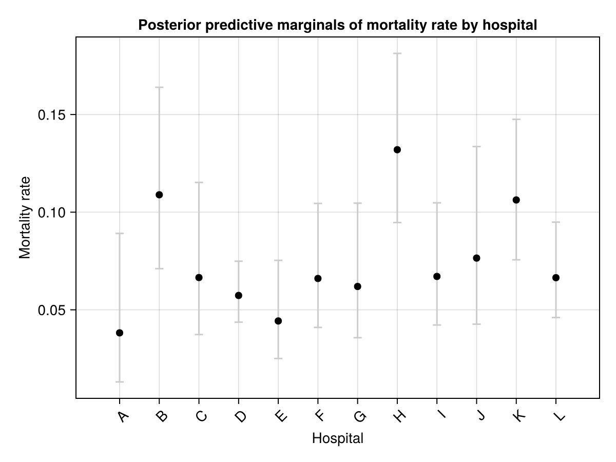
Hospital H stands out, with the highest fitted rate and an interval well above the others. The companion tutorial, Getting familiar with INLA, goes deeper on these accessors, on model-comparison criteria like DIC and WAIC, and on drawing joint posterior samples.

The same model through TMB

tmb runs the fast point-estimate engine: it finds the hyperparameter mode (the MAP) and fits a single Gaussian there, giving a MAP value and a standard error for each hyperparameter. Note that the model object is the same lgm, only the entry-point function changes:

tmb_result = tmb(lgm, surg_data.r)

TMBResult:
  Model: LatentGaussianModel{HyperparameterSpec{@NamedTuple{τ_u::Hyperparameter{Base.Fix1{typeof(broadcast), typeof(log)}, :natural}}, @NamedTuple{}}, Latte._PatternAugmentedLatentModel{Latte.RoutedLatentModel{CombinedModel{LinearSolve.CHOLMODFactorization{Nothing}}, @NamedTuple{τ_iid::Symbol}}, SparseArrays.SparseMatrixCSC{Int64, Int64}}, LinearlyTransformedObservationModel{Latte.BinomialTrialsObservationModel{ExponentialFamily{Distributions.Binomial, LogitLink, Nothing, Nothing}, Vector{Int64}}, SparseArrays.SparseMatrixCSC{Float64, Int64}, Nothing}}
  Hyperparameters (working-space MAP ± SE):
    τ_u       +1.2315 ± 0.4304
  Latent dimension: 13
  log p(y) ≈ -44.4584 (Laplace at MAP)
  Time: 7.13 s

The same accessors work on the result, returning the same Distributions.jl marginals. TMB's marginal for τ_u is a single Gaussian (in the working, here log, space) reported back on the natural scale, so its median is the MAP estimate and its spread the standard error:

τ_tmb = hyperparameter_marginals(tmb_result, :τ_u)[1]
median(τ_tmb), std(τ_tmb)

(3.4263545007688756, 1.6955013203257583)

TMB is exact when the hyperparameter posterior is close to Gaussian in the working (here log) space, which is often the case for well-identified models. Its single Gaussian cannot bend to follow a skewed posterior, though, which is the trade-off against INLA's grid.

The same model through HMC-Laplace

hmc_laplace keeps the inner Laplace approximation for the latent field but replaces the deterministic hyperparameter treatment with NUTS, sampling the hyperparameter posterior directly. It is the most faithful engine when that posterior is genuinely non-Gaussian, at the cost of running an MCMC chain. We seed the RNG for a reproducible chain:

using Random
hmc_result = hmc_laplace(
    lgm, surg_data.r; n_samples = 500, n_warmup = 200, rng = MersenneTwister(0)
)

HMCLaplaceResult:
  Model: LatentGaussianModel{HyperparameterSpec{@NamedTuple{τ_u::Hyperparameter{Base.Fix1{typeof(broadcast), typeof(log)}, :natural}}, @NamedTuple{}}, Latte._PatternAugmentedLatentModel{Latte.RoutedLatentModel{CombinedModel{LinearSolve.CHOLMODFactorization{Nothing}}, @NamedTuple{τ_iid::Symbol}}, SparseArrays.SparseMatrixCSC{Int64, Int64}}, LinearlyTransformedObservationModel{Latte.BinomialTrialsObservationModel{ExponentialFamily{Distributions.Binomial, LogitLink, Nothing, Nothing}, Vector{Int64}}, SparseArrays.SparseMatrixCSC{Float64, Int64}, Nothing}}
  θ samples: 500 (+ 200 warmup)
  Hyperparameters (posterior mean ± SD, natural space):
    τ_u       +3.4397 ± 1.4249
  Latent dimension: 13
  Diagnostics:
    accept rate:  0.857
    tree depth:   1.39 (mean)
    step size:    1.1945 (mean)
    divergences:  2
  Time: 3.47 s

Check that the chain behaved before trusting the marginals, then read τ_u back through the same accessor. Here the marginal is an empirical one built from the NUTS draws, summarised by its median and a 95% credible interval:

converged(hmc_result), divergences(hmc_result)

(true, 2)

τ_hmc = hyperparameter_marginals(hmc_result, :τ_u)[1]
median(τ_hmc), quantile(τ_hmc, 0.025), quantile(τ_hmc, 0.975)

(3.134720322240986, 1.1624724651789704, 6.974742920834128)

Which engine, when?

All three approximate the same posterior; they differ in how they handle the hyperparameters and therefore in speed and faithfulness.

• Reach for inla by default. It is fast and accurate on the great majority of latent Gaussian models, and it recovers the hyperparameter skew that TMB misses.

• Reach for tmb when you want the quickest fit and a MAP-plus-standard-error summary is enough, or when the model has many hyperparameters and you are content with empirical Bayes at the mode.

• Reach for hmc_laplace when the hyperparameter posterior is curved or strongly skewed (scale-versus-correlation trade-offs, parameters pinned against a boundary) and you need faithful tails, and there are few enough hyperparameters that sampling stays affordable.

The dedicated tutorials work each engine on a model built for its strengths: age-structured stock assessment (SAM) for TMB, and sampling hyperparameters for HMC-Laplace. The TMB and HMC-Laplace engine pages cover the methods and their tuning in more detail.

Conclusion

That covers the core workflow: write one @latte model, then run inla, tmb, or hmc_laplace on it and read the marginals back through the same accessor functions. Next, Getting familiar with INLA stays with this surgery model and digs into the result object: marginal accessors in depth, model-comparison criteria, and posterior sampling. The other tutorials build on this with spatial fields, temporal smoothing, custom likelihoods, and more.

References

INLA

Approximate Bayesian Inference for Latent Gaussian Models by Using Integrated Nested Laplace Approximations↗

H. Rue, S. Martino & N. Chopin

J. R. Statist. Soc. B · 2009 · doi:10.1111/j.1467-9868.2008.00700.x

The original INLA paper: deterministic approximate Bayesian inference for latent Gaussian models via nested Laplace approximations and numerical integration over the hyperparameters.

TMB

TMB: Automatic Differentiation and Laplace Approximation↗

K. Kristensen, A. Nielsen, C. W. Berg, H. Skaug & B. M. Bell

Journal of Statistical Software · 2016 · doi:10.18637/jss.v070.i05

The TMB R package: fast Laplace approximation of the marginal likelihood for latent-variable models, with automatic differentiation for the gradients and Hessians.

Embedded Laplace + HMC

Hamiltonian Monte Carlo using an Adjoint-differentiated Laplace Approximation↗

C. C. Margossian, A. Vehtari, D. Simpson & R. Agrawal

Advances in Neural Information Processing Systems (NeurIPS) · 2020 · arXiv:2004.12550

Hamiltonian Monte Carlo over the hyperparameters, with the latent Gaussian field marginalised by an embedded Laplace approximation and the gradient propagated through that inner solve. The method this engine implements.

---

This page was generated using Literate.jl.