Spatio-temporal disease surveillance

Disease incidence varies across both space and time. An additive model can capture where risk is high and when it peaks, but it assumes every region follows the same temporal trend. In practice spatial patterns often shift over time: an emerging epidemic may spread outward from a focus, or an intervention may reduce risk in some regions earlier than others.

This tutorial uses separable space-time models to capture those interactions. It covers how to specify a separable interaction in a @latte model, how the Kronecker-product structure Q_time ⊗ Q_space enforces smoothness in both dimensions at once, why a structured interaction term needs accompanying main effects, and how DIC, WAIC, and the marginal likelihood help choose between the fitted models.

Simulating spatio-temporal data

We work with a simulated disease surveillance scenario: case counts across a 5×5 grid of regions over 12 time periods. Using simulated data lets us know the truth and check whether the models recover it.

using Random, SparseArrays, Distributions, Statistics, DataFrames
Random.seed!(42)

n_rows, n_cols = 5, 5
n_regions = n_rows * n_cols  # 25
n_time = 12

12

First, we build a rook-adjacency matrix for the grid (each cell connects to its horizontal and vertical neighbours):

function grid_adjacency(nrow, ncol)
    n = nrow * ncol
    W = spzeros(n, n)
    for i in 1:nrow, j in 1:ncol
        node = (i - 1) * ncol + j
        if j < ncol  # right neighbour
            W[node, node + 1] = 1.0
            W[node + 1, node] = 1.0
        end
        if i < nrow  # bottom neighbour
            W[node, node + ncol] = 1.0
            W[node + ncol, node] = 1.0
        end
    end
    return W
end
W = grid_adjacency(n_rows, n_cols)

25×25 SparseArrays.SparseMatrixCSC{Float64, Int64} with 80 stored entries:
⎡⠪⡢⡈⠢⡀⠀⠀⠀⠀⠀⠀⠀⠀⎤
⎢⠢⡈⠠⡢⡈⠢⡀⠀⠀⠀⠀⠀⠀⎥
⎢⠀⠈⠢⡈⠊⡠⡈⠢⡀⠀⠀⠀⠀⎥
⎢⠀⠀⠀⠈⠢⡈⠪⠂⡈⠢⡀⠀⠀⎥
⎢⠀⠀⠀⠀⠀⠈⠢⡈⠪⡢⠈⠢⡀⎥
⎢⠀⠀⠀⠀⠀⠀⠀⠈⠢⡀⠪⡢⡀⎥
⎣⠀⠀⠀⠀⠀⠀⠀⠀⠀⠈⠀⠈⠀⎦

Now we simulate the ground truth. The linear predictor for region $r$ at time $t$ is

$${\eta }_{t,r}=\mu +u_r+v_t+{\delta }_{t,r}$$

where $u_r$ is a spatial gradient, $v_t$ is a temporal trend, and ${\delta }_{t,r}$ is a space-time interaction — a wave that sweeps across the grid over time.

intercept = 0.5

# Spatial effect: gradient from northwest (low) to southeast (high)
u_true = [(i + j) / (n_rows + n_cols) for i in 1:n_rows for j in 1:n_cols]
u_true .-= mean(u_true)
u_true .*= 0.6

# Temporal effect: inverted-U trend peaking around the middle
v_true = [-0.04 * (t - n_time / 2)^2 + 0.3 for t in 1:n_time]
v_true .-= mean(v_true)

# Interaction: a sinusoidal wave sweeping across the grid
delta_true = zeros(n_time, n_regions)
for t in 1:n_time
    for i in 1:n_rows, j in 1:n_cols
        r = (i - 1) * n_cols + j
        phase = (i + j) / (n_rows + n_cols)
        delta_true[t, r] = 0.4 * sin(2π * (t / n_time - phase))
    end
end

# Population at risk per region (gives expected counts of ~10–40)
pop = round.(Int, exp.(randn(n_regions) .* 0.3 .+ 3.0))

# Generate Poisson counts
df = DataFrame(time = Int[], region = Int[], y = Int[], expected = Float64[])
for t in 1:n_time, r in 1:n_regions
    η = intercept + u_true[r] + v_true[t] + delta_true[t, r]
    count = rand(Poisson(pop[r] * exp(η)))
    push!(df, (time = t, region = r, y = count, expected = Float64(pop[r])))
end
(observations = nrow(df), mean_count = round(mean(df.y), digits = 1))

(observations = 300, mean_count = 37.6)

Exploratory visualisation

A heatmap of the standardised rate (observed / expected) gives a first look at the space-time structure:

using CairoMakie

rate_matrix = reshape(df.y ./ df.expected, n_regions, n_time)'
fig = Figure(size = (800, 400))
ax = Axis(
    fig[1, 1],
    xlabel = "Region", ylabel = "Time period",
    title = "Standardised rate (observed / expected)"
)
hm = heatmap!(ax, 1:n_regions, 1:n_time, rate_matrix', colormap = Reverse(:RdYlBu))
Colorbar(fig[1, 2], hm)
fig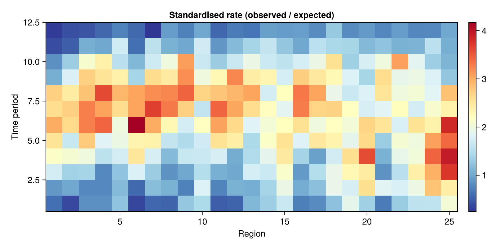

Both a spatial gradient (left vs right) and a temporal arc (middle rows brighter) are visible. The bright patch also shifts across regions over time, which is the interaction signal that an additive model cannot capture.

using Latte
using Distributions
using GaussianMarkovRandomFields: BesagModel, RWModel, SeparableModel
using LinearAlgebra

The three multi-hyperparameter models below share a set of inla keyword arguments: automatic exploration-strategy selection, a Gaussian latent marginalisation, and an explicit set of accumulator strategies. AutoExplorationStrategy matters most here. A Cartesian grid scales as (points-per-dim)^(n_hp), which is manageable for the 2-hyperparameter models but reaches hundreds of points for the 4-hyperparameter full_model. Auto keeps a grid in 2-D and switches to a Central Composite Design (~25 points) in 4-D. The strategies are immutable configs;inla() materialises them into fresh accumulator state on each call, so this tuple is safely reused.

const INLA_KWARGS = (
    progress = false,
    exploration_strategy = AutoExplorationStrategy(),
    latent_marginalization_method = GaussianMarginal(),
    accumulators = (
        DICStrategy(),
        MarginalLogLikelihoodStrategy(),
        WAICStrategy(),
    ),
)

(progress = false, exploration_strategy = AutoExplorationStrategy(GridExplorationStrategy(1.0, 2.5, 1), CCDExplorationStrategy(1.1)), latent_marginalization_method = GaussianMarginal(), accumulators = (DICStrategy(), MarginalLogLikelihoodStrategy(), WAICStrategy(15, :sample, 512)))

Model 1: Additive main effects

We start with a model that assumes spatial and temporal effects are independent:

$$\log {\lambda }_{t,r}=\mu +u_r+v_t$$

The spatial component is a Besag (ICAR) model and the temporal component is a first-order random walk, each with a PC prior on its precision:

@latte function additive_model(y, expected, region, time, n_regions, n_time, W)
    τ_besag ~ PCPrior.Precision(1.0, α = 0.01)
    τ_rw1 ~ PCPrior.Precision(1.0, α = 0.01)
    β ~ MvNormal(zeros(1), 100.0 * I(1))
    u ~ BesagModel(W; normalize_var = Val{true}())(τ = τ_besag)
    v ~ RWModel{1}(n_time)(τ = τ_rw1)
    for i in eachindex(y)
        y[i] ~ Poisson(
            expected[i] * exp(β[1] + u[region[i]] + v[time[i]])
        )
    end
end

lgm_add = additive_model(df.y, df.expected, df.region, df.time, n_regions, n_time, W)
result_additive = inla(lgm_add, df.y; INLA_KWARGS...)

INLAResult:
  Model: LatentGaussianModel{HyperparameterSpec{@NamedTuple{τ_besag::Hyperparameter{Bijectors.TruncatedBijector{Float64, Float64}, :natural}, τ_rw1::Hyperparameter{Bijectors.TruncatedBijector{Float64, Float64}, :natural}}, @NamedTuple{}}, Latte._PatternAugmentedLatentModel{Latte.RoutedLatentModel{CombinedModel{LinearSolve.CHOLMODFactorization{Nothing}}, @NamedTuple{τ_besag::Symbol, τ_rw1::Symbol}}, SparseArrays.SparseMatrixCSC{Int64, Int64}}, LinearlyTransformedObservationModel{ExponentialFamily{Distributions.Poisson, LogLink, Nothing, Nothing}, SparseArrays.SparseMatrixCSC{Float64, Int64}, Vector{Float64}}}
  Hyperparameters: 2
  Latent variables: 38
  Mode: (τ_besag=182.8161, τ_rw1=17.9767)
  Convergence: ✓
  Total time: 19.89 seconds
  Exploration: 16 points (16 integration)

Model comparison metrics:
Deviance Information Criterion (DIC):
  DIC: 2549.73
  Effective parameters (p_D): 0.48
  Mean deviance (D̄): 2549.25
  Deviance at mode: 2548.77

Marginal Log-Likelihood:
  log p(y): -1330.63

Watanabe-Akaike Information Criterion (WAIC):
  WAIC: 2660.7
  Effective parameters (p_WAIC): 85.33
  Log pointwise predictive density (lppd): -1245.02


Use .hyperparameter_marginals, .latent_marginals, .accumulators for analysis

The fitted rates come from observation_marginals, which reports fitted counts with the exposure included; dividing by expected recovers a relative-risk equivalent for the heatmap.

obs_add = observation_marginals(result_additive)
fit_add = summary_df(obs_add)
fitted_add = reshape(fit_add.median ./ df.expected, n_regions, n_time)'
fig = Figure(size = (800, 400))
ax = Axis(
    fig[1, 1],
    xlabel = "Region", ylabel = "Time period",
    title = "Additive model — fitted rates"
)
hm = heatmap!(ax, 1:n_regions, 1:n_time, fitted_add', colormap = Reverse(:RdYlBu))
Colorbar(fig[1, 2], hm)
fig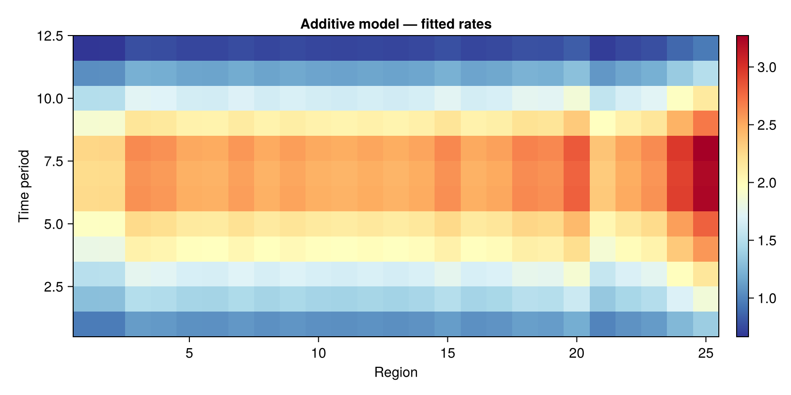

The additive model captures the overall spatial gradient and temporal arc, but the fitted surface is separable by construction — every region gets the same temporal pattern, just shifted up or down. It cannot reproduce the sweeping wave visible in the raw data.

Model 2: Interaction-only (a cautionary tale)

A tempting alternative is to replace the additive model with a single separable interaction term. Its precision matrix is a Kronecker product

$$Q=Q_{\text{time}}\otimes Q_{\text{space}}$$

With RWModel{1} for time and BesagModel(W) for space, this enforces smoothness in both dimensions at once. We try it here as the sole random effect.

The Separable field has size n_time × n_regions, flattened in row-major order (δ[(t-1)*n_regions + r] for region r at time t). This matches the kron(Q_time, Q_space) convention.

@latte function interaction_only_model(y, expected, region, time, n_regions, n_time, W)
    τ_rw1_separable ~ PCPrior.Precision(1.0, α = 0.01)
    τ_besag_separable ~ PCPrior.Precision(1.0, α = 0.01)
    β ~ MvNormal(zeros(1), 100.0 * I(1))
    δ ~ SeparableModel(
        RWModel{1}(n_time),
        BesagModel(W; normalize_var = Val{true}()),
    )(τ_rw1 = τ_rw1_separable, τ_besag = τ_besag_separable)
    for i in eachindex(y)
        δ_idx = (time[i] - 1) * n_regions + region[i]
        y[i] ~ Poisson(
            expected[i] * exp(β[1] + δ[δ_idx])
        )
    end
end

lgm_int_only = interaction_only_model(df.y, df.expected, df.region, df.time, n_regions, n_time, W)
result_interaction_only = inla(lgm_int_only, df.y; INLA_KWARGS...)

obs_int_only = observation_marginals(result_interaction_only)
fit_int_only = summary_df(obs_int_only)
fitted_int_only = reshape(fit_int_only.median ./ df.expected, n_regions, n_time)'
fig = Figure(size = (800, 400))
ax = Axis(
    fig[1, 1],
    xlabel = "Region", ylabel = "Time period",
    title = "Interaction-only model — fitted rates"
)
hm = heatmap!(ax, 1:n_regions, 1:n_time, fitted_int_only', colormap = Reverse(:RdYlBu))
Colorbar(fig[1, 2], hm)
fig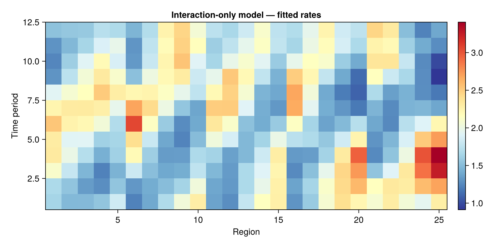

This model fits worse than the additive one. The fitted rates are over-smoothed and barely capture any structure.

Why interaction-only fails: the constraint story

The explanation lies in how the constraints of the two components compose under the Kronecker product.

Both the RW1 and the Besag components are rank-deficient: each carries a sum-to-zero constraint. Combining them through Q_time ⊗ Q_space makes those constraints compose. The RW1 part contributes $\sum _t{x}_{t,s}=0$ for each region $s$ (25 constraints), and the Besag part contributes $\sum _s{x}_{t,s}=0$ for each time $t$ (12 constraints, one of them redundant).

That leaves 36 constraints in total. The consequence that matters is that the Besag constraints force the spatial mean to zero at every time point. The interaction field ${\delta }_{t,r}$ then cannot carry any temporal main effect $v_t$ (which shifts all regions up or down together) or spatial main effect $u_r$ (which shifts all time points), so it represents pure interaction: deviations from additivity and nothing else.

With no separate main-effect terms for $u_r$ and $v_t$, the model is left trying to explain the entire signal through pure interaction, which it cannot do.

Model 3: Main effects + interaction (the right way)

The correct formulation adds the interaction term alongside main effects, following Knorr-Held's (2000) Type IV interaction structure:

$$\log {\lambda }_{t,r}=\mu +u_r+v_t+{\delta }_{t,r}$$

where $u_r\sim \text{Besag}$, $v_t\sim \text{RW1}$, and ${\delta }_{t,r}\sim \text{Separable}(\text{RW1},\text{Besag})$. The main effects absorb the marginal spatial and temporal patterns, freeing the interaction to capture only what changes across both dimensions:

@latte function full_model(y, expected, region, time, n_regions, n_time, W)
    τ_besag ~ PCPrior.Precision(1.0, α = 0.01)
    τ_rw1 ~ PCPrior.Precision(1.0, α = 0.01)
    τ_rw1_separable ~ PCPrior.Precision(1.0, α = 0.01)
    τ_besag_separable ~ PCPrior.Precision(1.0, α = 0.01)
    β ~ MvNormal(zeros(1), 100.0 * I(1))
    u ~ BesagModel(W; normalize_var = Val{true}())(τ = τ_besag)
    v ~ RWModel{1}(n_time)(τ = τ_rw1)
    δ ~ SeparableModel(
        RWModel{1}(n_time),
        BesagModel(W; normalize_var = Val{true}()),
    )(τ_rw1 = τ_rw1_separable, τ_besag = τ_besag_separable)
    for i in eachindex(y)
        δ_idx = (time[i] - 1) * n_regions + region[i]
        y[i] ~ Poisson(
            expected[i] * exp(β[1] + u[region[i]] + v[time[i]] + δ[δ_idx])
        )
    end
end

lgm_full = full_model(df.y, df.expected, df.region, df.time, n_regions, n_time, W)
result_full = inla(lgm_full, df.y; INLA_KWARGS...)

INLAResult:
  Model: LatentGaussianModel{HyperparameterSpec{@NamedTuple{τ_besag::Hyperparameter{Bijectors.TruncatedBijector{Float64, Float64}, :natural}, τ_rw1::Hyperparameter{Bijectors.TruncatedBijector{Float64, Float64}, :natural}, τ_rw1_separable::Hyperparameter{Bijectors.TruncatedBijector{Float64, Float64}, :natural}, τ_besag_separable::Hyperparameter{Bijectors.TruncatedBijector{Float64, Float64}, :natural}}, @NamedTuple{}}, Latte._PatternAugmentedLatentModel{Latte.RoutedLatentModel{CombinedModel{LinearSolve.CHOLMODFactorization{Nothing}}, @NamedTuple{τ_besag::Symbol, τ_rw1::Symbol, τ_rw1_separable::Symbol, τ_besag_separable::Symbol}}, SparseArrays.SparseMatrixCSC{Int64, Int64}}, LinearlyTransformedObservationModel{ExponentialFamily{Distributions.Poisson, LogLink, Nothing, Nothing}, SparseArrays.SparseMatrixCSC{Float64, Int64}, Vector{Float64}}}
  Hyperparameters: 4
  Latent variables: 338
  Mode: (τ_besag=163.5378, τ_rw1=16.4612, τ_rw1_separable=6.9688, τ_besag_separable=6.9703)
  Convergence: ✓
  Total time: 27.24 seconds
  Exploration: 25 points (25 integration)

Model comparison metrics:
Deviance Information Criterion (DIC):
  DIC: 1752.07
  Effective parameters (p_D): 0.77
  Mean deviance (D̄): 1751.3
  Deviance at mode: 1750.53

Marginal Log-Likelihood:
  log p(y): -1056.8

Watanabe-Akaike Information Criterion (WAIC):
  WAIC: 1923.6
  Effective parameters (p_WAIC): 59.71
  Log pointwise predictive density (lppd): -902.09


Use .hyperparameter_marginals, .latent_marginals, .accumulators for analysis

Let's see the fitted surface:

obs_full = observation_marginals(result_full)
fit_full = summary_df(obs_full)
fitted_full = reshape(fit_full.median ./ df.expected, n_regions, n_time)'
fig = Figure(size = (800, 400))
ax = Axis(
    fig[1, 1],
    xlabel = "Region", ylabel = "Time period",
    title = "Full model — fitted rates"
)
hm = heatmap!(ax, 1:n_regions, 1:n_time, fitted_full', colormap = Reverse(:RdYlBu))
Colorbar(fig[1, 2], hm)
fig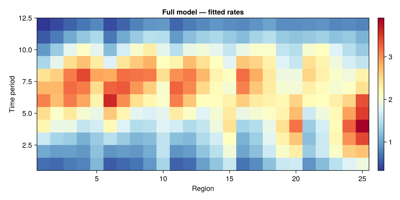

The full model recovers the shifting wave. Main effects handle the spatial gradient and temporal arc, and the interaction term adds the region-specific temporal deviations.

Spatial snapshots at selected time points

Spatial maps at four time points show the interaction directly. We reshape each time slice back into the 5×5 grid:

snapshot_times = [1, 4, 8, 12]

fig = Figure(size = (900, 250))
for (k, t) in enumerate(snapshot_times)
    local ax = Axis(
        fig[1, k],
        title = "t = $t",
        xlabel = k == 1 ? "Column" : "", ylabel = k == 1 ? "Row" : "",
        aspect = DataAspect()
    )
    rates = (fit_full.median ./ df.expected)[df.time .== t]
    grid = reshape(rates[sortperm(df.region[df.time .== t])], n_cols, n_rows)
    heatmap!(ax, 1:n_cols, 1:n_rows, grid, colormap = Reverse(:RdYlBu))
end
fig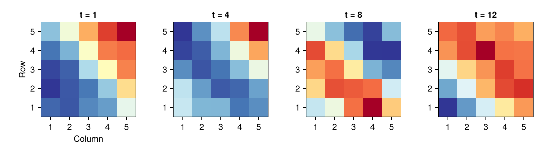

The high-risk area migrates across the grid over time, tracing the wave we simulated.

Side-by-side comparison

Let's put all three models next to each other:

fig = Figure(size = (1200, 400))
ax1 = Axis(
    fig[1, 1],
    xlabel = "Region", ylabel = "Time period",
    title = "Additive (main effects only)"
)
ax2 = Axis(
    fig[1, 2],
    xlabel = "Region", ylabel = "Time period",
    title = "Interaction only (no main effects)"
)
ax3 = Axis(
    fig[1, 3],
    xlabel = "Region", ylabel = "Time period",
    title = "Main effects + interaction"
)
heatmap!(ax1, 1:n_regions, 1:n_time, fitted_add', colormap = Reverse(:RdYlBu))
heatmap!(ax2, 1:n_regions, 1:n_time, fitted_int_only', colormap = Reverse(:RdYlBu))
heatmap!(ax3, 1:n_regions, 1:n_time, fitted_full', colormap = Reverse(:RdYlBu))
fig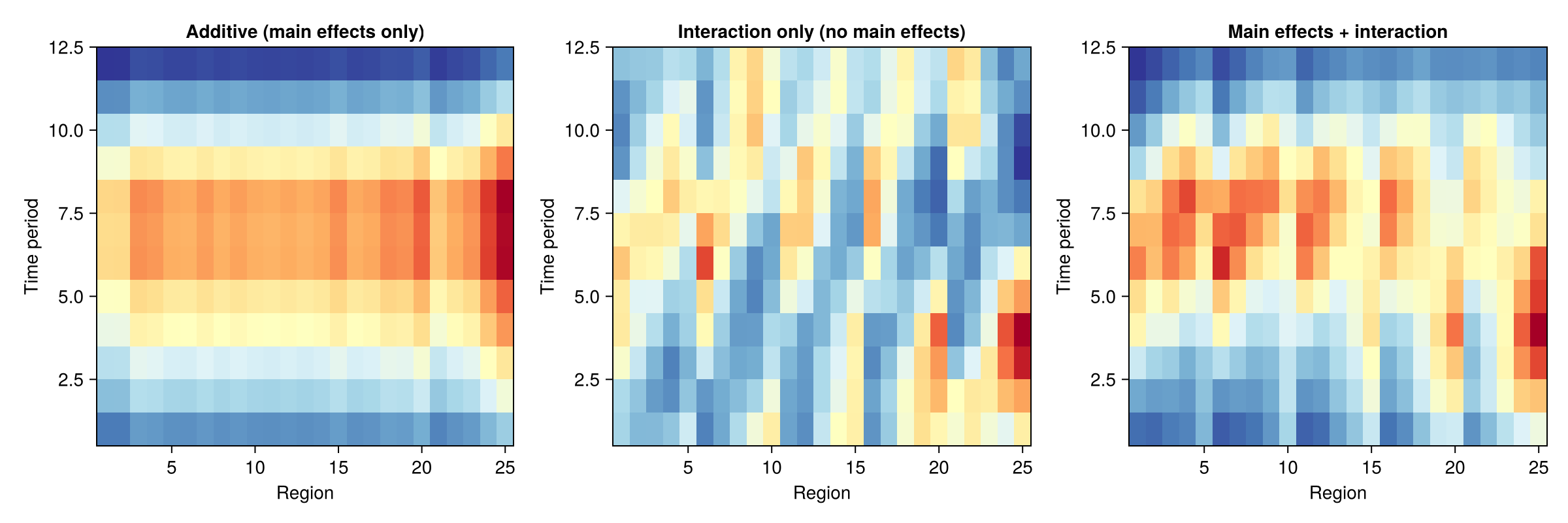

Model comparison

INLA computes several model comparison criteria as part of inference, and they land in result.accumulators. DIC and WAIC both weigh fit against complexity, with lower values preferred; the log marginal likelihood is a model-selection score where higher is preferred. The accumulator tuple we configured in INLA_KWARGS orders them as DIC, log marginal likelihood, then WAIC.

comparison = DataFrame(
    model = String[], DIC = Float64[], p_D = Float64[],
    WAIC = Float64[], log_ML = Float64[],
)
for (name, res) in [
        ("Additive", result_additive),
        ("Interaction only", result_interaction_only),
        ("Full (main+inter)", result_full),
    ]
    push!(
        comparison, (
            name,
            round(res.accumulators[1].DIC, digits = 1),
            round(res.accumulators[1].p_D, digits = 1),
            round(res.accumulators[3].WAIC, digits = 1),
            round(res.accumulators[2].log_marginal_likelihood, digits = 1),
        )
    )
end
comparison

3×5 DataFrame
 Row │ model              DIC      p_D      WAIC     log_ML
     │ String             Float64  Float64  Float64  Float64
─────┼───────────────────────────────────────────────────────
   1 │ Additive            2549.7      0.5   2660.7  -1330.6
   2 │ Interaction only    3065.9      1.2   3556.2  -1690.4
   3 │ Full (main+inter)   1752.1      0.8   1923.6  -1056.8

The full model leads on every criterion: lowest DIC and WAIC, highest marginal likelihood. The interaction-only model trails both others, confirming that a structured interaction term cannot substitute for main effects.

Hyperparameter posteriors

The full model has four hyperparameters. The summary table reads each marginal off the natural (declared) scale; we add a column naming the components in declared order:

hp_full = summary_df(hyperparameter_marginals(result_full))
insertcols!(hp_full, 1, :parameter => collect(keys(hyperparameter_groups(result_full))))

4×7 DataFrame
 Row │ parameter          mode       median     q2_5      q97_5     mean      std
     │ Symbol             Float64    Float64    Float64   Float64   Float64   Float64
─────┼─────────────────────────────────────────────────────────────────────────────────
   1 │ τ_besag            137.159    161.356    78.7935   329.705   172.491   64.7451
   2 │ τ_rw1               13.1278    15.5846    7.42648   32.3038   16.653    6.45709
   3 │ τ_rw1_separable      2.48941    6.96851   1.09966   44.1583   10.7707  11.1389
   4 │ τ_besag_separable    2.48995    6.97042   1.09998   44.1708   10.7737  11.1419

The main-effect precisions (${\tau }_{\text{besag}}$, ${\tau }_{\text{rw1}}$) control the smoothness of the spatial and temporal main effects. The interaction precisions (${\tau }_{\text{rw1,sep}}$, ${\tau }_{\text{besag,sep}}$) control the smoothness of the space-time deviations.

Summary

Separable space-time models capture interactions that additive models cannot, but they have to be specified correctly. The points worth keeping:

• An additive model assumes every region follows the same temporal pattern. It is simpler and works well when there is no space-time interaction.

• A separable interaction term uses a Kronecker product $Q_{\text{time}}\otimes Q_{\text{space}}$ to enforce smoothness in both dimensions while allowing region-specific temporal patterns.

• A structured spatial component like Besag imposes sum-to-zero constraints that make the interaction pure: it represents only deviations from additive structure, so the main effects have to be included separately to capture the marginal spatial and temporal patterns.

• SeparableModel(time_component, space_component) composes the two precision matrices via Kronecker product; inside the @latte block it lives on an n_time × n_regions flat vector indexed by (time-1)*n_regions + region.

• DIC, WAIC, and the marginal likelihood help decide whether the extra flexibility of the interaction model is justified by the data.

These models see use in spatial epidemiology, environmental monitoring, and other settings where spatial patterns evolve over time. For background on the interaction taxonomy (Types I–IV), see Knorr-Held (2000).

References

Knorr-Held

Bayesian Modelling of Inseparable Space-Time Variation in Disease Risk↗

L. Knorr-Held

Statistics in Medicine · 2000

Introduces the Type I–IV taxonomy of space-time interaction priors as Kronecker products of the spatial and temporal main-effect structures; the Type IV (Besag ⊗ RW) interaction used in the full model here.

Besag

Spatial Interaction and the Statistical Analysis of Lattice Systems↗

J. Besag

J. R. Statist. Soc. B · 1974 · doi:10.1111/j.2517-6161.1974.tb00999.x

The foundational paper on conditional autoregressive (CAR) models, the intrinsic Gaussian Markov random field that the spatial (Besag/ICAR) component is built from.

PC priors

Penalising Model Component Complexity: A Principled, Practical Approach to Constructing Priors↗

D. Simpson, H. Rue, A. Riebler, T. G. Martins & S. H. Sørbye

Statistical Science · 2017 · doi:10.1214/16-STS576

Penalised Complexity priors shrink each model component toward a simpler base model, with interpretable scaling such as P(σ > U) = α; the priors used on every precision hyperparameter here.

---

This page was generated using Literate.jl.