Nonlinear regression: Bayesian smoothing with INLA

When the relationship between a predictor and a response is nonlinear and of unknown form, we need a model flexible enough to adapt to the data without committing to a parametric shape. Generalized additive models (GAMs) are the usual frequentist tool, but they do not return full posterior uncertainty on the smoothness of the curve. Here we use INLA with a second-order random walk (RW2) prior, which gives a Bayesian counterpart to the smooth term in a GAM and propagates uncertainty about smoothness through to the fitted curve.

Along the way the tutorial covers:

• fitting a Gaussian observation model (our first one)

• using an RW2 prior as a nonparametric smooth, the discrete analogue of a cubic smoothing spline

• reading off the two hyperparameters, observation noise and RW2 precision, that jointly set the bias-variance tradeoff

• comparing the nonparametric fit against a linear baseline

The dataset

We use the mcycle dataset (Silverman, 1985): 133 accelerometer readings from a simulated motorcycle crash test. The response is head acceleration (in g) measured at various times (in milliseconds) after impact. It is a standard benchmark for nonparametric regression and turns up across the smoothing literature.

using DataFrames
times = [
    2.4, 2.6, 3.2, 3.6, 4.0, 6.2, 6.6, 6.8, 7.8, 8.2, 8.8, 8.8, 9.6,
    10.0, 10.2, 10.6, 11.0, 11.4, 13.2, 13.6, 13.8, 14.6, 14.6, 14.6,
    14.6, 14.6, 14.6, 14.8, 15.4, 15.4, 15.4, 15.4, 15.6, 15.6, 15.8,
    15.8, 16.0, 16.0, 16.2, 16.2, 16.2, 16.4, 16.4, 16.6, 16.8, 16.8,
    16.8, 17.6, 17.6, 17.6, 17.6, 17.8, 17.8, 18.6, 18.6, 19.2, 19.4,
    19.4, 19.6, 20.2, 20.4, 21.2, 21.4, 21.8, 22.0, 23.2, 23.4, 24.0,
    24.2, 24.2, 24.6, 25.0, 25.0, 25.4, 25.4, 25.6, 26.0, 26.2, 26.2,
    26.4, 27.0, 27.2, 27.2, 27.2, 27.6, 28.2, 28.4, 28.4, 28.6, 29.4,
    30.2, 31.0, 31.2, 32.0, 32.0, 32.8, 33.4, 33.8, 34.4, 34.8, 35.2,
    35.2, 35.4, 35.6, 35.6, 36.2, 36.2, 38.0, 38.0, 39.2, 39.4, 40.0,
    40.4, 41.6, 41.6, 42.4, 42.8, 42.8, 43.0, 44.0, 44.4, 45.0, 46.6,
    47.8, 47.8, 48.8, 50.6, 52.0, 53.2, 55.0, 55.0, 55.4, 57.6,
]
accel = [
    0.0, -1.3, -2.7, 0.0, -2.7, -2.7, -2.7, -1.3, -2.7, -2.7, -1.3,
    -2.7, -2.7, -2.7, -5.4, -2.7, -5.4, 0.0, -2.7, -2.7, 0.0, -13.3,
    -5.4, -5.4, -9.3, -16.0, -22.8, -2.7, -22.8, -32.1, -53.5, -54.9,
    -40.2, -21.5, -21.5, -50.8, -42.9, -26.8, -21.5, -50.8, -61.7, -5.4,
    -80.4, -59.0, -71.0, -91.1, -77.7, -37.5, -85.6, -123.1, -101.9,
    -99.1, -104.4, -112.5, -50.8, -123.1, -85.6, -72.3, -127.2, -123.1,
    -117.9, -134.0, -101.9, -108.4, -123.1, -123.1, -128.5, -112.5,
    -95.1, -81.8, -53.5, -64.4, -57.6, -72.3, -44.3, -26.8, -5.4,
    -107.1, -21.5, -65.6, -16.0, -45.6, -24.2, 9.5, 4.0, 12.0, -21.5,
    37.5, 46.9, -17.4, 36.2, 75.0, 8.1, 54.9, 48.2, 46.9, 16.0, 45.6,
    1.3, 75.0, -16.0, -54.9, 69.6, 34.8, 32.1, -37.5, 22.8, 46.9, 10.7,
    5.4, -1.3, -21.5, -13.3, 30.8, -10.7, 29.4, 0.0, -10.7, 14.7, -1.3,
    0.0, 10.7, 10.7, -26.8, -14.7, -13.3, 0.0, 10.7, -14.7, -2.7, 10.7,
    -2.7, 10.7,
];

The RW2 model needs integer-valued time indices. We rank the unique time values so the random walk operates on evenly spaced discrete positions.

unique_times = sort(unique(times))
time_to_idx = Dict(t => i for (i, t) in enumerate(unique_times))
time_idx = [time_to_idx[t] for t in times]
H = length(unique_times)

df = DataFrame(times = times, time_idx = time_idx, accel = accel)
first(df, 5)

5×3 DataFrame
 Row │ times    time_idx  accel
     │ Float64  Int64     Float64
─────┼────────────────────────────
   1 │     2.4         1      0.0
   2 │     2.6         2     -1.3
   3 │     3.2         3     -2.7
   4 │     3.6         4      0.0
   5 │     4.0         5     -2.7

Let's visualise the data:

using AlgebraOfGraphics, CairoMakie
draw(
    data(df) *
        mapping(:times => "Time after impact (ms)", :accel => "Head acceleration (g)") *
        visual(Scatter, markersize = 5, color = :gray40),
    axis = (title = "Motorcycle crash test: accelerometer data",),
)

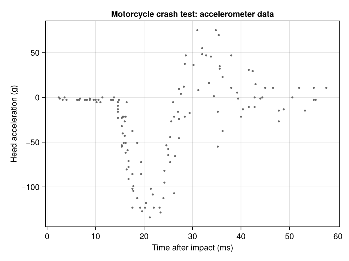
The acceleration trace is strongly nonlinear: a sharp negative spike around 15-25 ms, then a rebound and a damped oscillation. A low-order polynomial will not capture this shape, which is the setting nonparametric smoothing is built for, and where the Bayesian treatment buys us uncertainty on the estimated curve rather than a single point estimate.

Smoothing with random walks

A second-order random walk (RW2) places a Gaussian prior on the second differences of a discretized function:

$$f_{t+2}-2f_{t+1}+f_t\sim \mathcal{N}(0,{\tau }^{-1})$$

This penalizes the discretized second derivative, the same principle that underlies cubic smoothing splines; the RW2 prior is its discrete GMRF counterpart (Rue & Held, 2005). The precision $\tau$ plays the role of the smoothing parameter: a high $\tau$ forces the function towards a straight line (small second differences), while a low $\tau$ admits more curvature. In the Bayesian treatment $\tau$ is estimated from the data with its own posterior, rather than fixed by cross-validation.

Fitting the model

We model each observation as

$$y_i\sim \mathcal{N}({\mu }_i,{\sigma }^2),{\mu }_i={\beta }_0+f(t_i)$$

where ${\beta }_0$ is an intercept and $f$ is the RW2 smooth over time.

using Latte
using Distributions
using GaussianMarkovRandomFields: RWModel
using LinearAlgebra

@latte function rw2_smooth(y, time_idx, H)
    σ ~ PCPrior.Sigma(50.0, α = 0.01)
    τ_rw2 ~ PCPrior.Precision(1.0, α = 0.01)
    β ~ MvNormal(zeros(1), 100.0 * I(1))
    f ~ RWModel{2}(H)(τ = τ_rw2)
    for i in eachindex(y)
        y[i] ~ Normal(β[1] + f[time_idx[i]], σ)
    end
end

rw2_smooth (generic function with 1 method)

The model has two hyperparameters. The first, σ, is the observation-noise standard deviation; the PC prior PCPrior.Sigma(50.0, α = 0.01) puts only a 1% prior probability on the noise SD exceeding 50 g. The second, τ_rw2, is the RW2 precision, with a PC prior that penalises curvature relative to a linear baseline. Both are declared on their natural scale, so we read them back later without any transform.

Calling the @latte function builds the latent Gaussian model, which we then pass to inla:

lgm = rw2_smooth(df.accel, df.time_idx, H)
result = inla(lgm, df.accel; progress = false)

INLAResult:
  Model: LatentGaussianModel{HyperparameterSpec{@NamedTuple{σ::Hyperparameter{Base.Fix1{typeof(broadcast), typeof(log)}, :natural}, τ_rw2::Hyperparameter{Bijectors.TruncatedBijector{Float64, Float64}, :natural}}, @NamedTuple{}}, Latte._PatternAugmentedLatentModel{Latte.RoutedLatentModel{CombinedModel{LinearSolve.CHOLMODFactorization{Nothing}}, @NamedTuple{τ_rw2::Symbol}}, SparseArrays.SparseMatrixCSC{Int64, Int64}}, LinearlyTransformedObservationModel{ExponentialFamily{Distributions.Normal, IdentityLink, Nothing, Nothing}, SparseArrays.SparseMatrixCSC{Float64, Int64}, Nothing}}
  Hyperparameters: 2
  Latent variables: 95
  Mode: (σ=25.5132, τ_rw2=0.4884)
  Convergence: ✓
  Total time: 19.41 seconds
  Exploration: 17 points (17 integration)

Model comparison metrics:
Deviance Information Criterion (DIC):
  DIC: 1233.85
  Effective parameters (p_D): 0.96
  Mean deviance (D̄): 1232.9
  Deviance at mode: 1231.94

Marginal Log-Likelihood:
  log p(y): -645.3

Watanabe-Akaike Information Criterion (WAIC):
  WAIC: 1250.16
  Effective parameters (p_WAIC): 8.71
  Log pointwise predictive density (lppd): -616.37

Conditional Predictive Ordinates (CPO):
  LPML: -625.9
  Mean CPO: 0.0104
  Min CPO: 0.0003
  PIT computed: 133 values
  PIT mean: 0.4828 (ideal: 0.5)


Use .hyperparameter_marginals, .latent_marginals, .accumulators for analysis

Visualizing the fit

The observation marginals give us the posterior distribution of ${\mu }_i$, the expected acceleration at each observed time. Let's plot the posterior median with a 95% credible band:

obs = observation_marginals(result)
fit = summary_df(obs)
fit.times = df.times;

layers =
    data(df) * mapping(:times, :accel) *
    visual(Scatter, color = :gray70, markersize = 5) +
    data(fit) * mapping(:times, :q2_5, :q97_5) *
    visual(Band, color = (:steelblue, 0.25)) +
    data(fit) * mapping(:times, :median) *
    visual(Lines, color = :steelblue, linewidth = 2)
draw(
    layers,
    axis = (
        xlabel = "Time after impact (ms)", ylabel = "Head acceleration (g)",
        title = "RW2 smooth: posterior fit with 95% credible band",
    ),
)

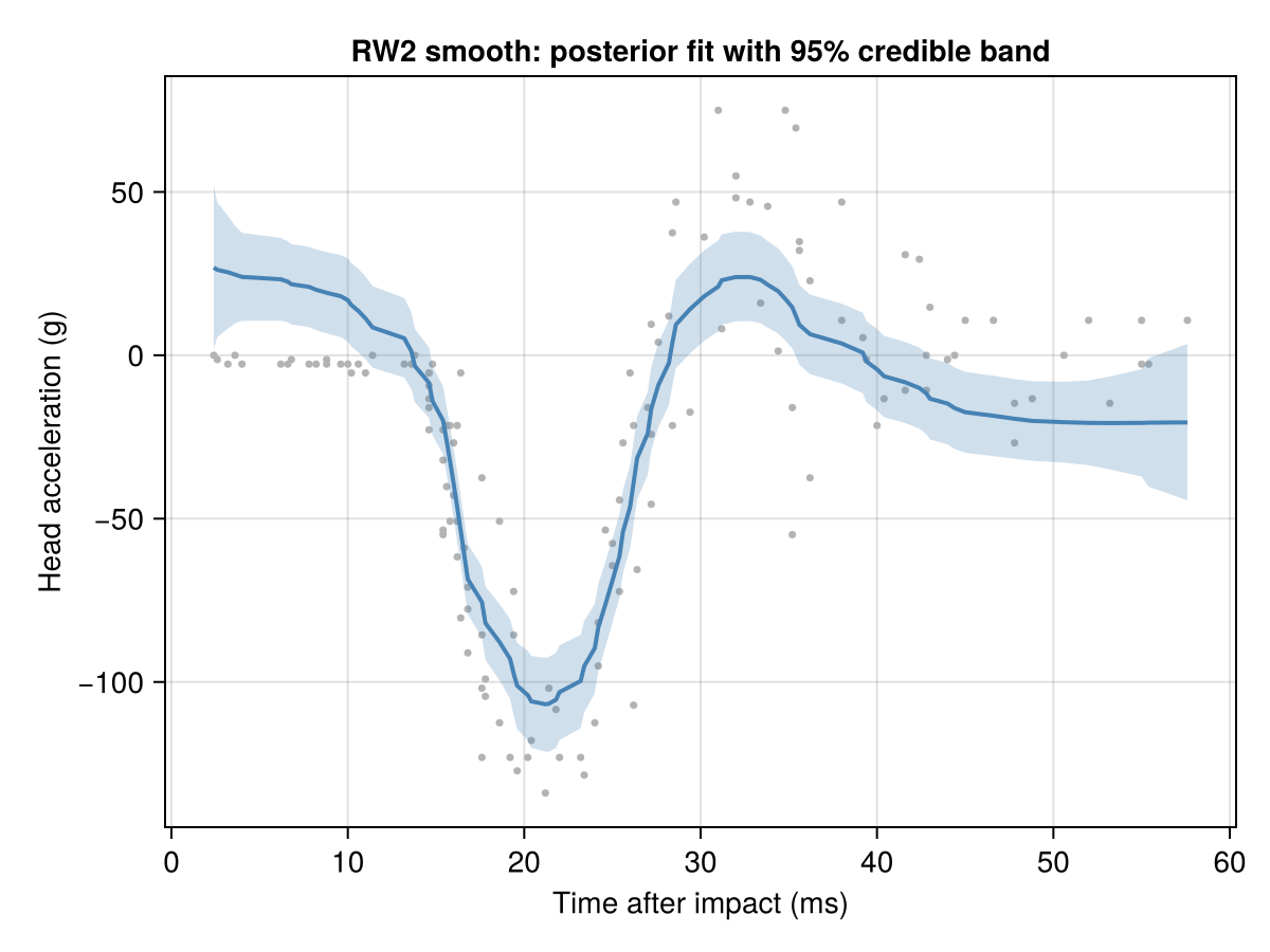
The smooth tracks the sharp deceleration spike and the subsequent rebound, and the band narrows where the data is dense and the mean curve is well-determined. One point is worth stressing: the band shows uncertainty in the mean function $\mu (t)$, not a prediction interval for new observations. Since $y_i\sim N({\mu }_i,{\sigma }^2)$ with $\sigma \approx 25$ g, individual readings scatter well beyond it. The posterior predictive check at the end of the tutorial gives the wider interval that folds in observation noise.

Hyperparameter posteriors

The two hyperparameters have distinct roles. The noise standard deviation $\sigma$ controls how much variation we attribute to measurement error, while the RW2 precision ${\tau }_{\text{rw2}}$ controls how smooth the underlying curve is. Their ratio determines the effective bias-variance tradeoff: high $\tau /{\sigma }^2$ favours a smooth curve, while low $\tau /{\sigma }^2$ lets the curve track the data more closely.

# Evaluate each marginal's density on a grid spanning its 0.1%–99.9% quantiles,
# then stack into one tidy frame faceted by hyperparameter.
function density_df(dist, label)
    xs = range(quantile(dist, 0.001), quantile(dist, 0.999); length = 200)
    return DataFrame(x = xs, density = pdf.(Ref(dist), xs), parameter = label)
end
hp_density = vcat(
    density_df(hyperparameter_marginals(result, :σ)[1], "Observation noise σ"),
    density_df(hyperparameter_marginals(result, :τ_rw2)[1], "RW2 precision τ_rw2"),
)
data(hp_density) *
    mapping(:x => "value", :density => "Density", layout = :parameter) *
    visual(Lines) |> draw(; facet = (; linkxaxes = :none))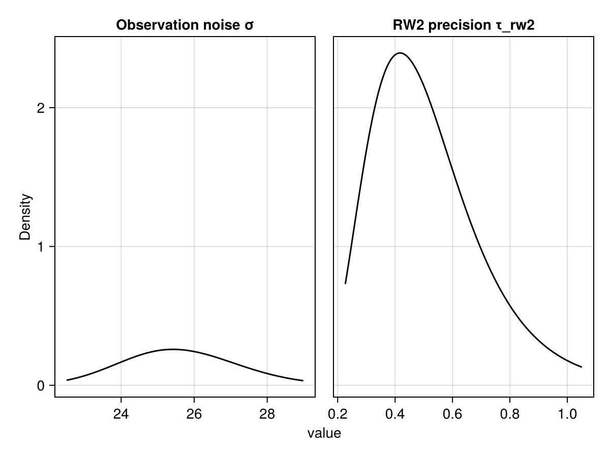

And the summary statistics for the two hyperparameters:

summary_df(hyperparameter_marginals(result))

2×6 DataFrame
 Row │ mode       median     q2_5       q97_5      mean       std
     │ Float64    Float64    Float64    Float64    Float64    Float64
─────┼────────────────────────────────────────────────────────────────
   1 │ 25.4177    25.5606    22.98      28.4486    25.6065    1.43104
   2 │  0.417311   0.484057   0.253166   0.927277   0.512386  0.17573

Comparison with a linear model

For a baseline, fit a straight-line mean ${\mu }_i={\beta }_0+{\beta }_1{t}_i$ with the same Gaussian noise and compare it against the smooth:

@latte function linear_model(y, x)
    σ ~ PCPrior.Sigma(50.0, α = 0.01)
    β ~ MvNormal(zeros(2), 100.0 * I(2))
    for i in eachindex(y)
        y[i] ~ Normal(β[1] + β[2] * x[i], σ)
    end
end

lgm_linear = linear_model(df.accel, df.times)
result_linear = inla(lgm_linear, df.accel; progress = false)

INLAResult:
  Model: LatentGaussianModel{HyperparameterSpec{@NamedTuple{σ::Hyperparameter{Base.Fix1{typeof(broadcast), typeof(log)}, :natural}}, @NamedTuple{}}, Latte._PatternAugmentedLatentModel{Latte.RoutedLatentModel{FixedEffectsModel{LinearSolve.DiagonalFactorization, Nothing}, @NamedTuple{}}, SparseArrays.SparseMatrixCSC{Int64, Int64}}, LinearlyTransformedObservationModel{ExponentialFamily{Distributions.Normal, IdentityLink, Nothing, Nothing}, SparseArrays.SparseMatrixCSC{Float64, Int64}, Nothing}}
  Hyperparameters: 1
  Latent variables: 2
  Mode: (σ=46.8956)
  Convergence: ✓
  Total time: 9.80 seconds
  Exploration: 5 points (5 integration)

Model comparison metrics:
Deviance Information Criterion (DIC):
  DIC: 1404.58
  Effective parameters (p_D): 0.92
  Mean deviance (D̄): 1403.66
  Deviance at mode: 1402.74

Marginal Log-Likelihood:
  log p(y): -715.2

Watanabe-Akaike Information Criterion (WAIC):
  WAIC: 1407.12
  Effective parameters (p_WAIC): 1.89
  Log pointwise predictive density (lppd): -701.66

Conditional Predictive Ordinates (CPO):
  LPML: -703.59
  Mean CPO: 0.006
  Min CPO: 0.0005
  PIT computed: 133 values
  PIT mean: 0.4902 (ideal: 0.5)


Use .hyperparameter_marginals, .latent_marginals, .accumulators for analysis

Let's overlay both fits:

obs_linear = observation_marginals(result_linear)
fit_linear = summary_df(obs_linear)
fit_linear.times = df.times;

# Stack the two posterior-median curves into one long frame, coloured by model.
fits = vcat(
    DataFrame(times = fit_linear.times, median = fit_linear.median, model = "Linear"),
    DataFrame(times = fit.times, median = fit.median, model = "RW2 smooth"),
)
layers =
    data(df) * mapping(:times, :accel) *
    visual(Scatter, color = :gray70, markersize = 5) +
    data(fits) * mapping(:times, :median, color = :model => "") *
    visual(Lines, linewidth = 2)
draw(
    layers,
    axis = (
        xlabel = "Time after impact (ms)", ylabel = "Head acceleration (g)",
        title = "Linear model vs RW2 smooth",
    ),
)

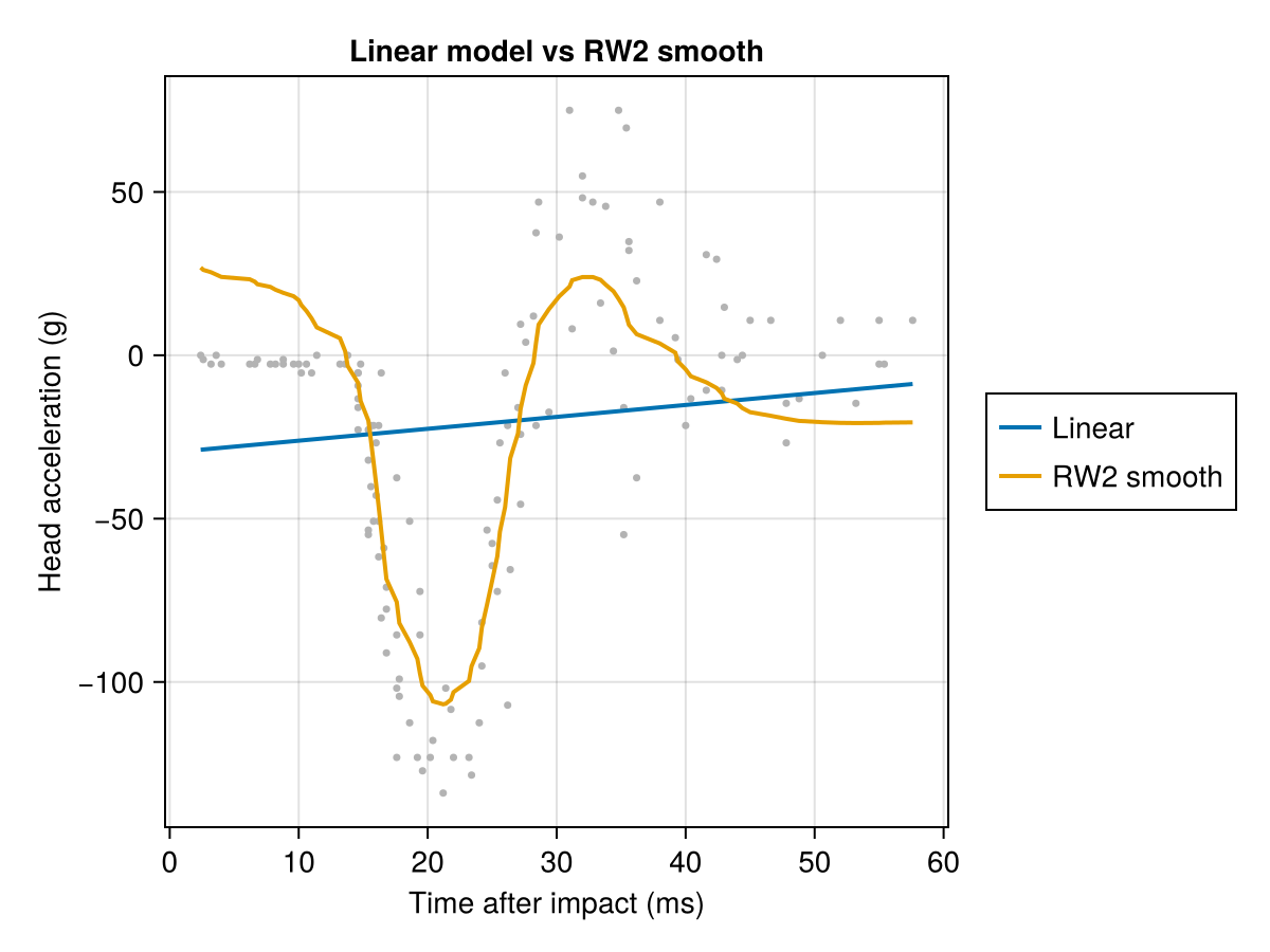
The linear model misses the nonlinear structure entirely. The default accumulators give us DIC, WAIC, and the log marginal likelihood to put numbers on the difference. We collect them into a small table:

comparison = DataFrame(
    model = ["Linear", "RW2"],
    DIC = [res.accumulators[1].DIC for res in (result_linear, result)],
    p_D = [res.accumulators[1].p_D for res in (result_linear, result)],
    WAIC = [res.accumulators[3].WAIC for res in (result_linear, result)],
    log_ML = [log_marginal_likelihood(res) for res in (result_linear, result)],
)

2×5 DataFrame
 Row │ model   DIC      p_D       WAIC     log_ML
     │ String  Float64  Float64   Float64  Float64
─────┼──────────────────────────────────────────────
   1 │ Linear  1404.58  0.920225  1407.12  -715.199
   2 │ RW2     1233.85  0.956855  1250.16  -645.303

Every criterion favours the RW2 model by a wide margin. Its effective number of parameters ($p_D$) is much larger, reflecting the extra flexibility, and the data justify that complexity rather than penalising it.

Posterior predictive check

To check that the model reproduces the variability in the data, we draw from the posterior predictive and see whether the observations fall inside it. rand(result, n; include_y = true) returns joint draws whose y field is an n × n_obs matrix of replicated responses:

using Random
Random.seed!(42)

n_obs = nrow(df)
n_samples = 200
pp = rand(result, n_samples; include_y = true).y
size(pp)

(200, 133)

For each observation, take the 2.5th and 97.5th percentiles of the replicated values across draws (one column per observation):

pp_df = DataFrame(
    times = df.times,
    accel = df.accel,
    pp_lo = [quantile(pp[:, i], 0.025) for i in 1:n_obs],
    pp_hi = [quantile(pp[:, i], 0.975) for i in 1:n_obs],
)

layers =
    data(pp_df) * mapping(:times, :pp_lo, :pp_hi) *
    visual(Band, color = (:steelblue, 0.2)) +
    data(pp_df) * mapping(:times, :accel) *
    visual(Scatter, color = :gray40, markersize = 4)
draw(
    layers,
    axis = (
        xlabel = "Time after impact (ms)", ylabel = "Head acceleration (g)",
        title = "Posterior predictive check",
    ),
)

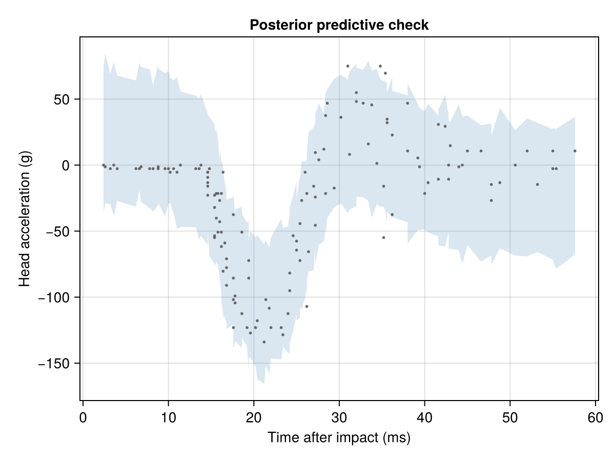
The observed data sit inside the predictive bands, so the model accounts for both the mean structure and the spread.

Summary

We fitted a nonlinear regression to the motorcycle crash data with INLA, using a Gaussian observation model and an RW2 smooth. A few points are worth carrying forward.

The second-order random walk prior is the discrete analogue of a cubic smoothing spline: it penalises second differences and yields a smooth curve that adapts to the data. The Gaussian family adds an observation-noise parameter $\sigma$ next to the smoothness precision $\tau$, and together they set the bias-variance tradeoff between structure attributed to the curve and variation attributed to noise. INLA estimates both from the data and returns full posterior uncertainty, so the smoothness is inferred rather than tuned by cross-validation. This gives a Bayesian counterpart to a frequentist GAM (mgcv::gam() in R), with posterior uncertainty on both the fitted curve and the degree of smoothness.

Natural extensions from here include heteroscedastic noise models, additive models with several smooth terms, and spatial smoothing via the SPDE approach.

References

Smoothing spline

Some Aspects of the Spline Smoothing Approach to Non-Parametric Regression Curve Fitting↗

B. W. Silverman

J. R. Statist. Soc. B · 1985 · doi:10.1111/j.2517-6161.1985.tb01327.x

Spline smoothing for non-parametric regression, and the source of the motorcycle-crash accelerometer dataset used here.

RW2

Gaussian Markov Random Fields: Theory and Applications↗

H. Rue & L. Held

Chapman & Hall/CRC · 2005 · doi:10.1201/9780203492024

The reference on GMRFs, including the random-walk priors (RW1/RW2) that act as discrete smoothing splines for the latent field.

PC priors

Penalising Model Component Complexity: A Principled, Practical Approach to Constructing Priors↗

D. Simpson, H. Rue, A. Riebler, T. G. Martins & S. H. Sørbye

Statistical Science · 2017 · doi:10.1214/16-STS576

Penalised-complexity (PC) priors: weakly informative priors that shrink a model component towards a simpler base model, used here for both the noise SD and the RW2 precision.

GAM

Generalized Additive Models: An Introduction with R (2nd ed.)↗

S. N. Wood

Chapman & Hall/CRC · 2017 · doi:10.1201/9781315370279

Generalized additive models and their penalised-spline smooths, the frequentist counterpart (mgcv::gam) to the Bayesian RW2 smooth fitted here.

---

This page was generated using Literate.jl.