Posterior predictive checks

A fitted model implies a distribution over datasets like the one we saw. A posterior predictive check draws new datasets from that distribution and asks whether they resemble the observed data. Where they diverge, the model is missing something.

Latte provides three functions for this workflow. posterior_predictive(result, n) draws n replicate datasets, ppc_stat(T, y, y_rep) evaluates a test statistic on the observed data and each replicate, and bayesian_pvalue(T, y, y_rep) returns the tail probability of the observed statistic under the replicates. The posterior predictive check and its Bayesian p-value go back to Gelman, Meng & Stern (1996).

Here we fit a plain Poisson model to data that is in fact overdispersed, and use a check to expose the misfit.

using Latte
using Distributions
using GaussianMarkovRandomFields: IIDModel
using Random, Statistics
using CairoMakie

Random.seed!(20260424)

Random.TaskLocalRNG()

Generate overdispersed counts

We simulate from a Negative-Binomial chosen to share the Poisson mean but carry larger variance, the usual signature of overdispersion.

n = 80
μ_true = exp.(randn(n) .* 0.3 .+ 1.5)
y = rand.(NegativeBinomial.(2.0, 2.0 ./ (2.0 .+ μ_true)))
println("n = $n, observed mean = $(round(mean(y), digits = 2)), var = $(round(var(y), digits = 2))")

n = 80, observed mean = 4.94, var = 20.49

Fit a Poisson model (deliberately wrong)

@latte function poisson_fit(y, n)
    τ ~ PCPrior.Precision(1.0, α = 0.01)
    x ~ IIDModel(n)(τ = τ)
    for i in eachindex(y)
        y[i] ~ Poisson(exp(x[i]))
    end
end
lgm = poisson_fit(y, n)
result = inla(lgm, y; progress = false)

INLAResult:
  Model: LatentGaussianModel{HyperparameterSpec{@NamedTuple{τ::Hyperparameter{Bijectors.TruncatedBijector{Float64, Float64}, :natural}}, @NamedTuple{}}, Latte._PatternAugmentedLatentModel{Latte.RoutedLatentModel{IIDModel{LinearSolve.DiagonalFactorization, Nothing, Nothing}, @NamedTuple{τ::Symbol}}, SparseArrays.SparseMatrixCSC{Int64, Int64}}, LinearlyTransformedObservationModel{ExponentialFamily{Distributions.Poisson, LogLink, Nothing, Nothing}, SparseArrays.SparseMatrixCSC{Float64, Int64}, Nothing}}
  Hyperparameters: 1
  Latent variables: 80
  Mode: (τ=0.4621)
  Convergence: ✓
  Total time: 13.20 seconds
  Exploration: 5 points (5 integration)

Model comparison metrics:
Deviance Information Criterion (DIC):
  DIC: 249.94
  Effective parameters (p_D): 0.15
  Mean deviance (D̄): 249.79
  Deviance at mode: 249.64

Marginal Log-Likelihood:
  log p(y): -251.14

Watanabe-Akaike Information Criterion (WAIC):
  WAIC: 346.3
  Effective parameters (p_WAIC): 25.45
  Log pointwise predictive density (lppd): -147.7

Conditional Predictive Ordinates (CPO):
  LPML: -10209.7
  Mean CPO: 0.0
  Min CPO: 0.0
  Unreliable observations: 80 / 80
  Max failure score: 130.17
  PIT computed: 80 values
  PIT mean: 0.5622 (ideal: 0.5)


Approximation quality (KLD):
  Max SKLD: 0.0349 (variable 24)
  Mean SKLD: 0.0025

Use .hyperparameter_marginals, .latent_marginals, .accumulators for analysis

Draw posterior predictive datasets

y_rep = posterior_predictive(result, 1000)
println("y_rep shape: ", size(y_rep))

y_rep shape: (1000, 80)

Check a few statistics

We look at three statistics: the mean, the standard deviation, and the maximum. A well-specified model reproduces all three. A Poisson fit to overdispersed counts should match the mean while underestimating the spread and the upper tail.

stats = [("mean", mean), ("std", std), ("maximum", maximum)]

fig = Figure(size = (900, 300))
for (k, (name, T)) in enumerate(stats)
    T_obs, T_rep = ppc_stat(T, y, y_rep)
    p = bayesian_pvalue(T, y, y_rep)
    local ax = Axis(
        fig[1, k], xlabel = name, ylabel = "count",
        title = "$name — Bayesian p = $(round(p, digits = 3))"
    )
    hist!(ax, T_rep, bins = 30, color = (:steelblue, 0.6))
    vlines!(ax, [T_obs], color = :red, linewidth = 2)
end
fig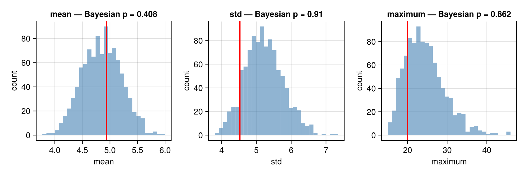

In each panel the red line is the observed statistic and the histogram is its posterior predictive distribution under the Poisson fit. The mean sits well inside the replicated distribution, with a p-value near 0.5, so the Poisson captures the location. The standard deviation and the maximum fall outside their histograms: the fitted Poisson generates data that is less variable and shorter-tailed than what we observed.

A p-value near 0 or 1 flags that the model is mis-specified for that aspect of the data. The remedy here is a likelihood that admits overdispersion, such as a Negative-Binomial or an observation-level random effect.

Choosing statistics

These checks are qualitative, and the Bayesian p-values are not calibrated, but a statistic landing far from 0.5 is a reliable hint of misfit. Choose statistics that target the behaviour you want the model to capture, whether that is tails, zero counts, autocorrelation, or group-level moments, rather than reaching only for the mean and standard deviation.

References

PPC

Posterior Predictive Assessment of Model Fitness via Realized Discrepancies↗

A. Gelman, X.-L. Meng & H. Stern

Statistica Sinica · 1996

Introduces posterior predictive checks and the Bayesian p-value: comparing a test statistic of the observed data against its distribution over datasets replicated from the fitted posterior to assess model fitness.

---

This page was generated using Literate.jl.