
Barrier Models: Spatial Fields That Respect Coastlines
A stationary spatial field correlates two locations by the straight-line distance between them. For a marine quantity such as fish abundance, salinity, or a pollutant, that assumption breaks down near a coastline. Two points on opposite sides of a peninsula are close as the crow flies, but a fish cannot swim through land. A stationary Matérn field smooths across the land anyway, borrowing strength between water bodies that are physically disconnected. Bakka et al. (2019) call this the coastline problem.
The barrier model addresses it. It is a non-stationary variant of the Matérn SPDE (Lindgren, Rue & Lindström, 2011) in which designated barrier regions (land) are given a tiny correlation range, so the field decorrelates sharply across them. Correlation then flows around the coast through water rather than straight across the land, while keeping the same sparse precision structure and computational cost. The barrier range is a fixed fraction of the water range, not a quantity we infer, so the model adds no extra hyperparameter.
In this tutorial we map a fish-abundance surface around the Florida peninsula, which separates two basins: the Gulf of Mexico to the west and the Atlantic to the east, connected only around the Keys to the south. The plan is to
download a real coastline and tag the land triangles of a mesh as barriers,
simulate a survey whose true abundance hot spot sits in the Gulf,
fit the same log-Gaussian Cox process twice, once with a barrier field and once with a stationary Matérn field, and
check, on held-out data, whether the stationary model bleeds the Gulf hot spot across the peninsula into the Atlantic.
The model
At survey station
where
Downloading a real coastline
We need a land polygon to decide which mesh triangles are barriers. Natural Earth provides public-domain land vectors; we pull the 1:10m GeoJSON (the same source the earthquake-intensity tutorial uses for its coastline) and cache it.
using Downloads

const NE_URL = "https://raw.githubusercontent.com/nvkelso/natural-earth-vector/" *
    "master/geojson/ne_10m_land.geojson"
geojson_path = joinpath(tempdir(), "ne_10m_land.geojson")
isfile(geojson_path) || Downloads.download(NE_URL, geojson_path)
filesize(geojson_path)10157965GeoJSON stores each landmass as one or more closed coordinate rings. We only need the rings near Florida, and we only ever test mesh-triangle centroids against them, so we never have to clip the large North-America polygon. We keep every ring whose bounding box overlaps our region.
Two parsing details are worth flagging. The North-America ring has ~66k vertices, and a single regex over the whole file backtracks catastrophically and silently drops it, so we split on the ring delimiter ]],[[ first and scan each chunk separately. A handful of Natural Earth coordinates also use scientific notation (e.g. 6.8e-05), so the number pattern must allow it.
function extract_rings(geojson_str::AbstractString, bbox; pad = 2.0)
    lon0, lat0, lon1, lat1 = bbox
    num = raw"-?\d+(?:\.\d+)?(?:[eE][-+]?\d+)?"
    coord_re = Regex("\\[\\s*($num)\\s*,\\s*($num)\\s*\\]")
    rings = Vector{Vector{Tuple{Float64, Float64}}}()
    # `Base.split` qualified: `DynamicPPL` (loaded later) also exports `split`.
    for chunk in Base.split(geojson_str, "]],[[")
        pts = Tuple{Float64, Float64}[]
        rlon0 = Inf; rlon1 = -Inf; rlat0 = Inf; rlat1 = -Inf
        for c in eachmatch(coord_re, chunk)
            lon = parse(Float64, c.captures[1])
            lat = parse(Float64, c.captures[2])
            push!(pts, (lon, lat))
            rlon0 = min(rlon0, lon); rlon1 = max(rlon1, lon)
            rlat0 = min(rlat0, lat); rlat1 = max(rlat1, lat)
        end
        if length(pts) > 2 &&
                rlon1 >= lon0 - pad && rlon0 <= lon1 + pad &&
                rlat1 >= lat0 - pad && rlat0 <= lat1 + pad
            push!(rings, pts)
        end
    end
    return rings
end

# (lon0, lat0, lon1, lat1): a window over Florida with open water on both
# sides, the Gulf of Mexico to the west and the Atlantic to the east.
const BBOX = (-87.0, 24.0, -78.0, 31.0)
land_rings = extract_rings(read(geojson_path, String), BBOX)
println("kept $(length(land_rings)) land ring(s) overlapping the region")
kept 216 land ring(s) overlapping the regionBuilding the mesh and tagging barriers
The barrier model lives on a triangular finite-element mesh, like the stationary Matérn SPDE. We lay a structured triangular grid over the whole window, covering both water and land, because the latent field is defined on every mesh node; the barrier only changes how the precision matrix is assembled over the land triangles.
Loading Ferrite, FerriteGmsh, Gmsh, LibGEOS activates the FEM machinery in GaussianMarkovRandomFields. We do not actually mesh anything with Gmsh here, as a uniform grid plus a land polygon is all the barrier model needs, but the extension is gated behind those packages being present.
using GaussianMarkovRandomFields
using Ferrite, FerriteGmsh, Gmsh, LibGEOS

# A coarse, fast mesh (~800 nodes); the window is wider E–W than N–S, so we use
# more cells along longitude. The Florida peninsula spans several cells, so the
# barrier never "leaks" through a one-cell gap.
const NX, NY = 32, 26
lon0, lat0, lon1, lat1 = BBOX
# `Vec` is exported by both Ferrite and CairoMakie, so we qualify it.
grid = generate_grid(Triangle, (NX, NY), Ferrite.Vec(lon0, lat0), Ferrite.Vec(lon1, lat1))
disc = FEMDiscretization(grid, Lagrange{RefTriangle, 1}(), QuadratureRule{RefTriangle}(2))
FEMDiscretization
grid: Ferrite.Grid{2, Ferrite.Triangle, Float64} with 1664 Ferrite.Triangle cells and 891 nodes
interpolation: Ferrite.Lagrange{Ferrite.RefTriangle, 1}()
quadrature_rule: Ferrite.QuadratureRule{Ferrite.RefTriangle, Vector{Float64}, Vector{Tensors.Vec{2, Float64}}}
# constraints: 0barrier_triangles(disc, polygon) returns the ids of triangles whose centroid lies inside polygon. We run it for each land ring and take the union.
barrier_cells = let s = Set{Int}()
    for ring in land_rings
        union!(s, barrier_triangles(disc, ring))
    end
    sort!(collect(s))
end

n_mesh = ndofs(disc)
println("mesh nodes: ", n_mesh)
println(
    "land (barrier) triangles: ", length(barrier_cells),
    " / ", length(grid.cells),
    "  (", round(100 * length(barrier_cells) / length(grid.cells), digits = 1), "%)"
)
mesh nodes: 891
land (barrier) triangles: 397 / 1664 (23.9%)Let's look at the tagged land. We will reuse this point-in-polygon test throughout to tell water from land.
function in_land(lon, lat, rings)
    inside = false
    for ring in rings
        n = length(ring)
        j = n
        for i in 1:n
            xi, yi = ring[i]
            xj, yj = ring[j]
            if ((yi > lat) != (yj > lat)) &&
                    (lon < (xj - xi) * (lat - yi) / (yj - yi) + xi)
                inside = !inside
            end
            j = i
        end
    end
    return inside
end

using CairoMakie

# Triangle centroids, coloured by whether they were tagged as barriers.
cell_centroids = [
    (
            sum(grid.nodes[n].x[1] for n in c.nodes) / length(c.nodes),
            sum(grid.nodes[n].x[2] for n in c.nodes) / length(c.nodes),
        )
        for c in grid.cells
]
is_barrier = falses(length(grid.cells))
is_barrier[barrier_cells] .= true

fig = Figure(size = (560, 480))
ax = Axis(
    fig[1, 1]; title = "Mesh triangles: water vs. barrier (land)",
    xlabel = "Longitude", ylabel = "Latitude", aspect = DataAspect()
)
scatter!(
    ax, [c[1] for c in cell_centroids], [c[2] for c in cell_centroids];
    color = [b ? :saddlebrown : :steelblue for b in is_barrier], markersize = 6
)
for ring in land_rings
    lines!(ax, [p[1] for p in ring], [p[2] for p in ring]; color = :black, linewidth = 1)
end
xlims!(ax, lon0, lon1); ylims!(ax, lat0, lat1)
fig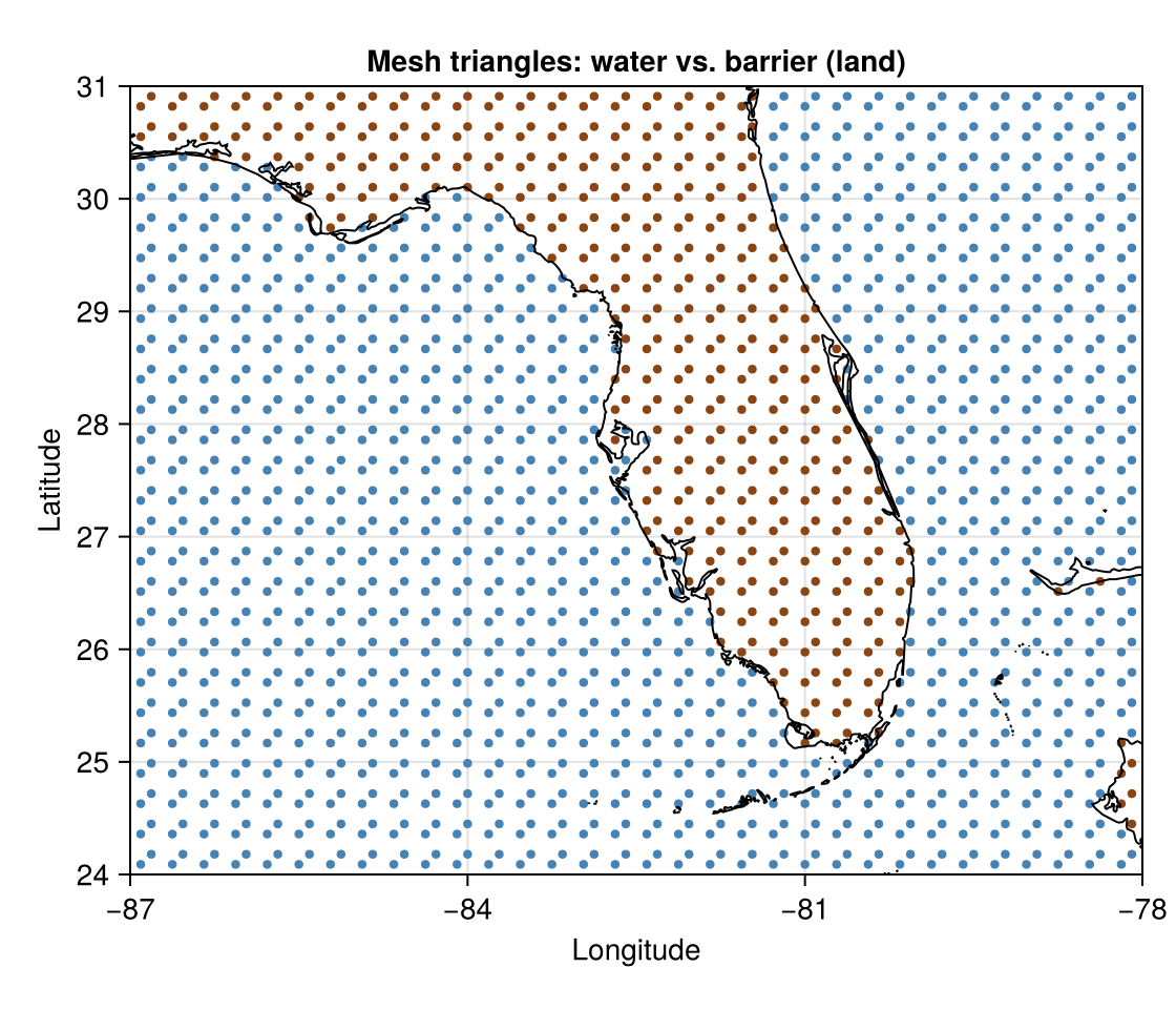
The brown triangles are the Florida peninsula (plus the mainland to the north-west and the Bahamas to the east); the blue triangles are the Gulf and the Atlantic. The peninsula is a solid, multi-cell-wide wall between the two basins.
A barrier-respecting ground truth
To judge the two models we need a known truth. We place a single abundance hot spot, think of a spawning ground, in the Gulf just off the west-central coast, and let its influence decay through water. The barrier field's own covariance expresses "influence that travels around the coast, not across it": a column of its covariance matrix, read off from the hot-spot node, is high near the hot spot, falls off through the Gulf, and is essentially zero on the Atlantic side of the peninsula.
This is the situation barrier models are designed for, a field whose correlation respects the coastline. The rest of the tutorial asks which model recovers it from noisy survey counts.
using LinearAlgebra, SparseArrays, Statistics, Random

const TRUE_RANGE = 2.5    # spatial range of the truth, in degrees (≈ 1/4 of the window)
true_field_model = BarrierModel(disc; barrier_cells = barrier_cells, range_fraction = 0.1)

# Node index of the hot spot (Gulf side, central-west coast).
mesh_coords = [grid.nodes[i].x for i in 1:length(grid.nodes)]
findnode(p) = argmin([(c[1] - p[1])^2 + (c[2] - p[2])^2 for c in mesh_coords])
hotspot = (-83.5, 28.5)
i_hot = findnode(hotspot)

# One covariance column = Q⁻¹ eₕₒₜ. Normalise to a 0–1 "influence" kernel.
Q_true = sparse(precision_matrix(true_field_model; τ = 1.0, range = TRUE_RANGE))
e_hot = zeros(n_mesh); e_hot[i_hot] = 1.0
kernel = Q_true \ e_hot
kernel = max.(kernel, 0.0)
kernel ./= maximum(kernel)

# True log-intensity on the mesh nodes: a background level plus the hot spot.
const TRUE_INTERCEPT = 0.0   # background intensity exp(0) = 1 count per station
const TRUE_AMP = 3.0         # hot-spot peak ≈ exp(3) ≈ 20 counts
true_log_intensity = TRUE_INTERCEPT .+ TRUE_AMP .* kernel;
Simulating the survey
Our research vessel only worked the Gulf shelf and never sampled the Atlantic side. We scatter survey stations over the water west of the peninsula, then draw a Poisson count at each from the true intensity. We also reserve two held-out sets to score predictions later: extra Gulf stations (a control, where both models have nearby data) and Atlantic stations (the test, separated from every survey station by land).
Random.seed!(20260613)

# Uniformly sample water points, then route them into survey / control / test.
function sample_water_points(n; rng, lon_lo, lon_hi, lat_lo = lat0 + 0.3, lat_hi = lat1 - 0.3)
    pts = Tuple{Float64, Float64}[]
    while length(pts) < n
        lon = lon_lo + (lon_hi - lon_lo) * rand(rng)
        lat = lat_lo + (lat_hi - lat_lo) * rand(rng)
        in_land(lon, lat, land_rings) || push!(pts, (lon, lat))
    end
    return pts
end
rng = MersenneTwister(1)

# Gulf = west of the peninsula; Atlantic = east of it (north of the Keys).
survey_pts = sample_water_points(140; rng, lon_lo = -86.5, lon_hi = -82.5)
gulf_test_pts = sample_water_points(40; rng, lon_lo = -86.5, lon_hi = -82.5)
atlantic_test_pts = sample_water_points(40; rng, lon_lo = -79.9, lon_hi = -79.0, lat_lo = 27.0, lat_hi = 30.5)

# Project the true mesh field to any set of points, then draw Poisson counts.
true_log_at(points) = evaluation_matrix(disc, reduce(vcat, [collect(p)' for p in points])) * true_log_intensity
draw_counts(points; rng) = [rand(rng, Poisson(exp(li))) for li in true_log_at(points)]

using Distributions
survey_counts = draw_counts(survey_pts; rng)
gulf_test_counts = draw_counts(gulf_test_pts; rng)
atlantic_test_counts = draw_counts(atlantic_test_pts; rng)

println(
    "survey stations: ", length(survey_pts),
    "   counts: min ", minimum(survey_counts), ", max ", maximum(survey_counts),
    ", mean ", round(mean(survey_counts), digits = 2)
)
survey stations: 140 counts: min 0, max 18, mean 3.11Let's see what the vessel collected, over the true intensity surface.
survey_mat = reduce(vcat, [collect(p)' for p in survey_pts])
A_obs = evaluation_matrix(disc, survey_mat)

# A fine grid for plotting the true surface (land masked out).
n_fine = 80
fine_lons = range(lon0 + 0.05, lon1 - 0.05; length = n_fine)
fine_lats = range(lat0 + 0.05, lat1 - 0.05; length = n_fine)
fine_pts = [(lon, lat) for lat in fine_lats, lon in fine_lons]
fine_mat = reduce(vcat, [collect(p)' for p in vec(fine_pts)])
A_fine = evaluation_matrix(disc, fine_mat)
water_mask = [in_land(lon, lat, land_rings) ? NaN : 1.0 for lat in fine_lats, lon in fine_lons]

true_surface = reshape(exp.(A_fine * true_log_intensity), n_fine, n_fine) .* water_mask

fig = Figure(size = (620, 520))
ax = Axis(
    fig[1, 1]; title = "True abundance + Gulf survey (counts)",
    xlabel = "Longitude", ylabel = "Latitude", aspect = DataAspect()
)
hm = heatmap!(ax, collect(fine_lons), collect(fine_lats), permutedims(true_surface); colormap = :viridis)
for ring in land_rings
    lines!(ax, [p[1] for p in ring], [p[2] for p in ring]; color = :white, linewidth = 1)
end
scatter!(
    ax, [p[1] for p in survey_pts], [p[2] for p in survey_pts];
    color = survey_counts, colormap = :inferno, strokewidth = 0.4, strokecolor = :white, markersize = 8
)
xlims!(ax, lon0, lon1); ylims!(ax, lat0, lat1)
Colorbar(fig[1, 2], hm; label = "intensity (expected count)")
fig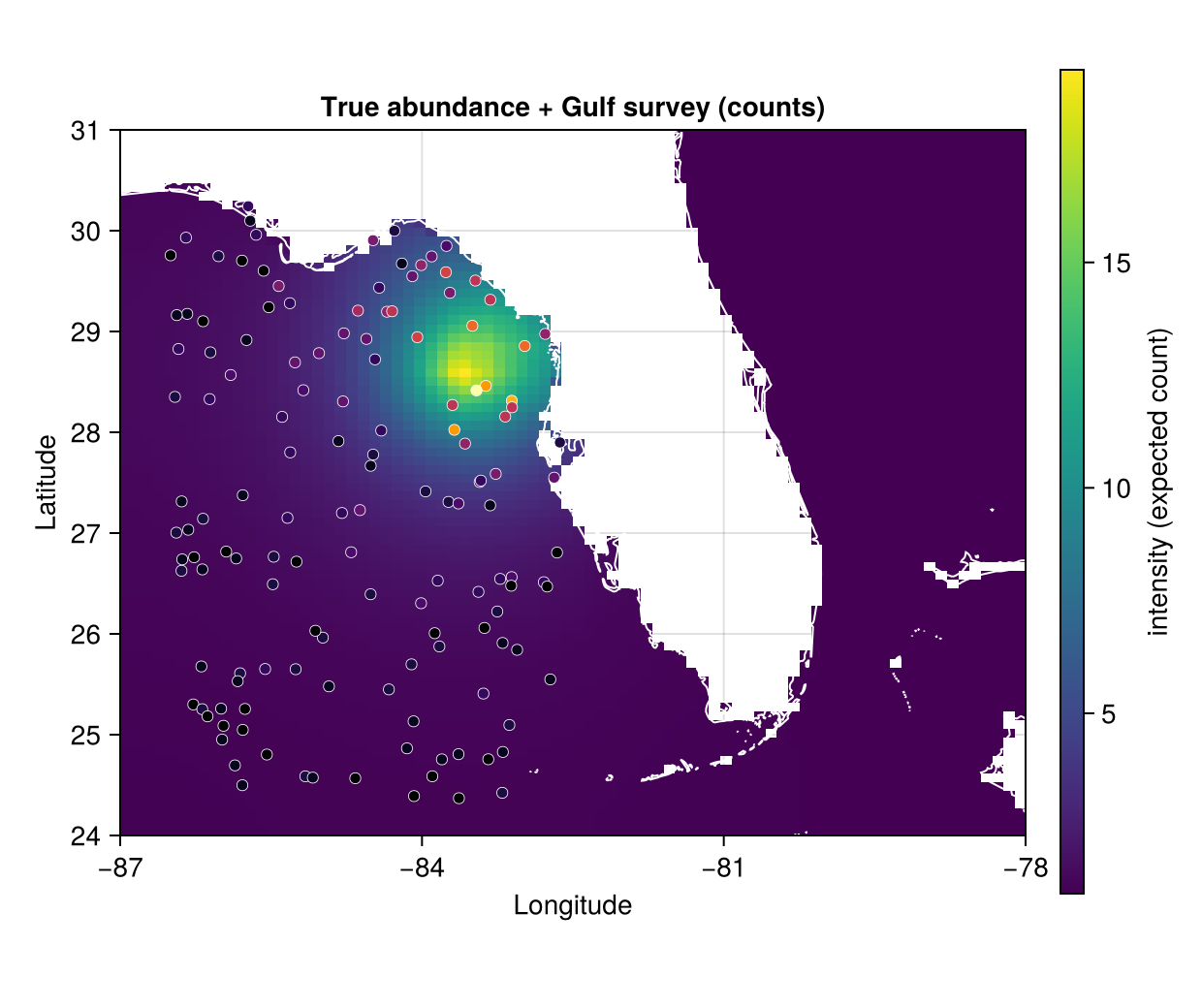
The hot spot sits in the Gulf; the survey covers the Gulf shelf and captures it. The Atlantic side is true background, and it goes unobserved.
Fitting the two models
Now the inference. We write the log-Gaussian Cox process once as a @latte model that takes the latent field's prior base as an argument, then fit it with each prior. The intercept gets a vague Gaussian prior, the field precision a penalised-complexity prior, and the spatial range a weakly informative Exponential.
using Latte

@latte function fish_lgcp(counts, base, A)
    β ~ MvNormal(zeros(1), 100.0 * I(1))
    τ ~ PCPrior.Precision(1.0, α = 0.01)
    spatial_range ~ Exponential(3.0)
    field ~ base(τ = τ, range = spatial_range)
    η = β[1] .+ A * field
    for i in eachindex(counts)
        counts[i] ~ Poisson(exp(η[i]))
    end
end
fish_lgcp (generic function with 1 method)The barrier prior tags the Florida land triangles. The stationary Matérn (smoothness = 0, the ν = 1 case the barrier model generalises) is the same field with no barriers. We fit both with SimplifiedLaplace latent marginals, whose skewness correction matters for count data and especially at the many zero-count stations.
barrier_prior = BarrierModel(disc; barrier_cells = barrier_cells, range_fraction = 0.1)
matern_prior = MaternModel(disc; smoothness = 0)

result_barrier = inla(
    fish_lgcp(survey_counts, barrier_prior, A_obs), survey_counts;
    progress = false, latent_marginalization_method = SimplifiedLaplace(),
)
result_matern = inla(
    fish_lgcp(survey_counts, matern_prior, A_obs), survey_counts;
    progress = false, latent_marginalization_method = SimplifiedLaplace(),
)
summary_df(hyperparameter_marginals(result_barrier))
2×6 DataFrame
Row │ mode median q2_5 q97_5 mean std
│ Float64 Float64 Float64 Float64 Float64 Float64
─────┼───────────────────────────────────────────────────────
1 │ 2.17117 2.51037 1.20915 4.46637 2.60467 0.881386
2 │ 3.37347 3.93915 2.50588 7.04259 4.16948 1.20069Both models infer the field precision τ and the spatial range. The barrier range fraction is fixed at construction (0.1) rather than inferred, so the two models estimate exactly the same parameters.
Predicted intensity surfaces
We evaluate each fitted field on the fine grid via linear_combinations, which assembles the posterior of
pred_barrier = linear_combinations(result_barrier; β = 1.0, field = A_fine)
pred_matern = linear_combinations(result_matern; β = 1.0, field = A_fine);

intensity_barrier = reshape(exp.(mean.(pred_barrier)), n_fine, n_fine) .* water_mask
intensity_matern = reshape(exp.(mean.(pred_matern)), n_fine, n_fine) .* water_mask

# Shared colour scale so the two panels are directly comparable.
cmax = maximum(filter(!isnan, vcat(vec(intensity_barrier), vec(intensity_matern))))

fig = Figure(size = (1080, 520))
for (col, (ttl, surf)) in enumerate(
        ("Barrier model" => intensity_barrier, "Stationary Matérn" => intensity_matern)
    )
    local ax = Axis(
        fig[1, col]; title = ttl, xlabel = "Longitude",
        ylabel = col == 1 ? "Latitude" : "", aspect = DataAspect()
    )
    local hm = heatmap!(
        ax, collect(fine_lons), collect(fine_lats), permutedims(surf);
        colormap = :viridis, colorrange = (0, cmax)
    )
    for ring in land_rings
        lines!(ax, [p[1] for p in ring], [p[2] for p in ring]; color = :white, linewidth = 1)
    end
    scatter!(
        ax, [p[1] for p in survey_pts], [p[2] for p in survey_pts];
        color = :white, markersize = 3
    )
    xlims!(ax, lon0, lon1); ylims!(ax, lat0, lat1)
    col == 2 && Colorbar(fig[1, 3], hm; label = "predicted intensity")
end
fig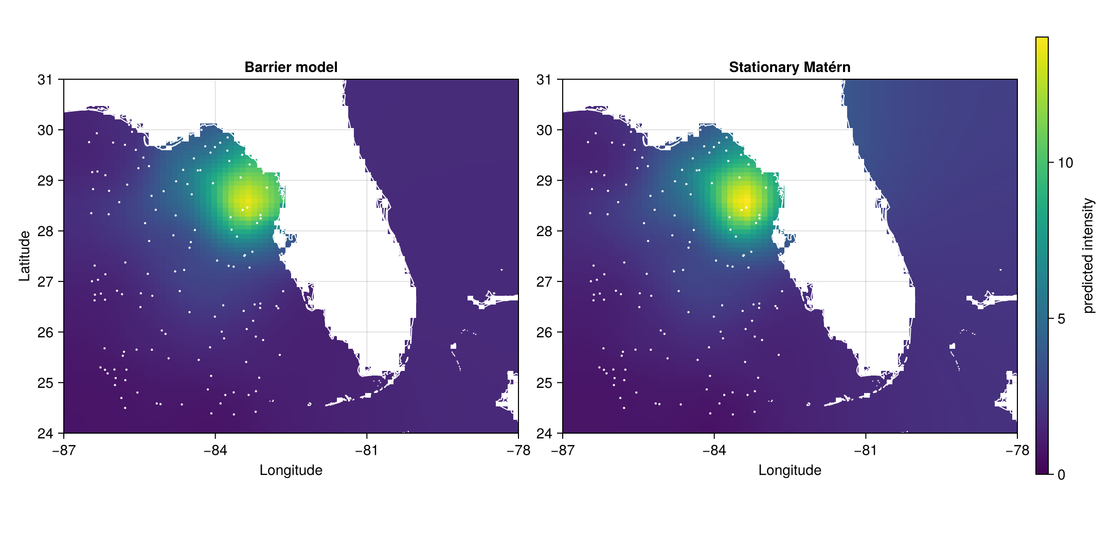
Both models agree in the Gulf, where the data live. The difference is on the Atlantic coast, directly east of the hot spot. The stationary Matérn smooths the high Gulf intensity straight across the peninsula, predicting a phantom hot spot in water it has no evidence for. The barrier model does not carry signal across the land, so the Atlantic stays at its background level, which is the truth.
Where each model is confident
The same contrast appears in the posterior uncertainty. We map the posterior standard deviation of the log-intensity.
sd_barrier = reshape(std.(pred_barrier), n_fine, n_fine) .* water_mask
sd_matern = reshape(std.(pred_matern), n_fine, n_fine) .* water_mask
sdmax = maximum(filter(!isnan, vcat(vec(sd_barrier), vec(sd_matern))))

fig = Figure(size = (1080, 520))
for (col, (ttl, surf)) in enumerate(
        ("Barrier model" => sd_barrier, "Stationary Matérn" => sd_matern)
    )
    local ax = Axis(
        fig[1, col]; title = "$ttl — posterior SD", xlabel = "Longitude",
        ylabel = col == 1 ? "Latitude" : "", aspect = DataAspect()
    )
    local hm = heatmap!(
        ax, collect(fine_lons), collect(fine_lats), permutedims(surf);
        colormap = :magma, colorrange = (0, sdmax)
    )
    for ring in land_rings
        lines!(ax, [p[1] for p in ring], [p[2] for p in ring]; color = :white, linewidth = 1)
    end
    xlims!(ax, lon0, lon1); ylims!(ax, lat0, lat1)
    col == 2 && Colorbar(fig[1, 3], hm; label = "posterior SD (log-intensity)")
end
fig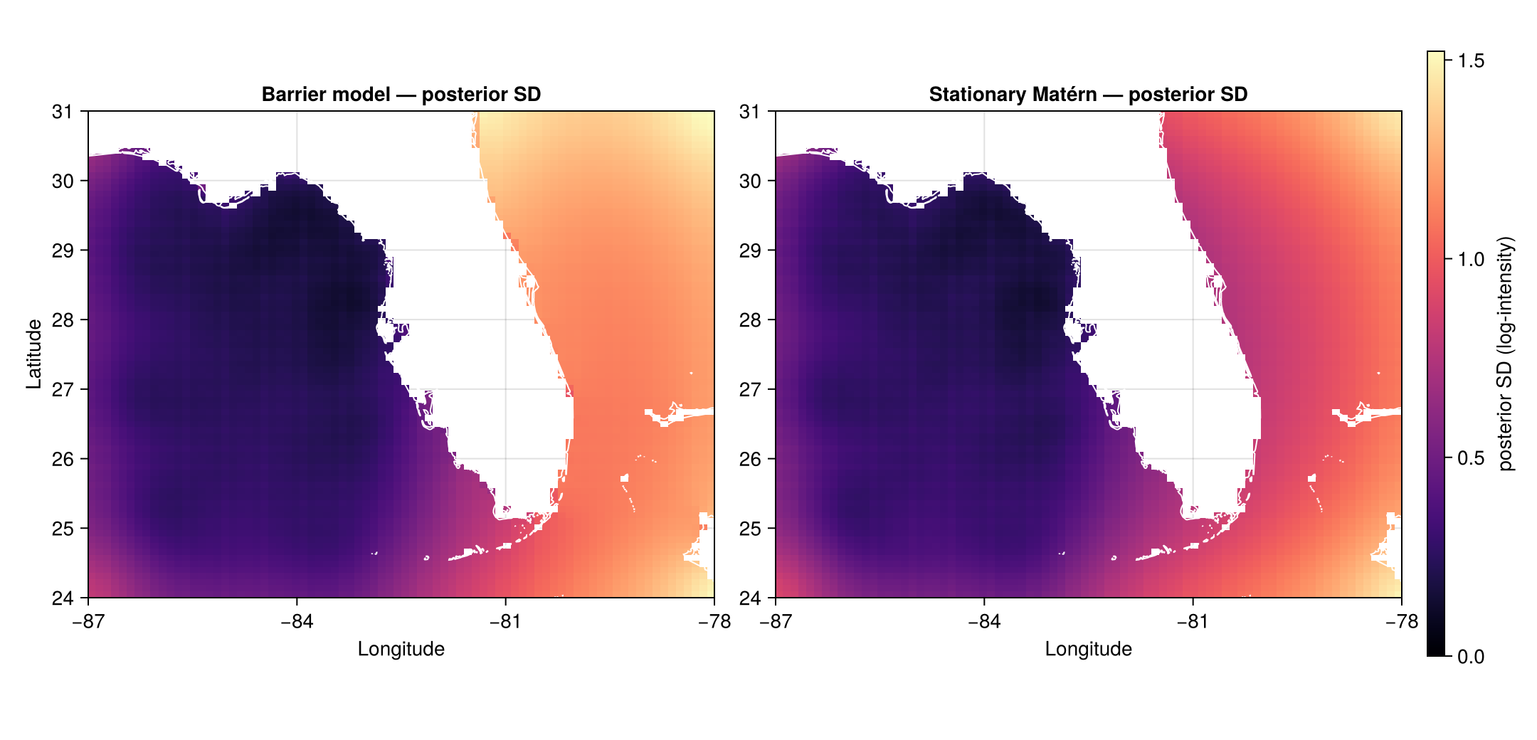
Both models report low posterior SD over the surveyed Gulf and high SD across the unobserved Atlantic, so neither pretends to know the field where it has no data. The more telling difference is quantitative rather than visual. Across the barrier, the stationary model is the more confident of the two, even though its mean is badly wrong. We turn to that next.
Quantitative validation on held-out data
Visual intuition is one thing; let's score it against the known truth on the held-out stations. For each we report the RMSE of the predicted log-intensity, the mean predicted intensity (the truth is ≈ 1.9 in the Gulf test region and ≈ 1.0 in the Atlantic), and the mean posterior standard deviation.
function score(result, points)
    A = evaluation_matrix(disc, reduce(vcat, [collect(p)' for p in points]))
    preds = linear_combinations(result; β = 1.0, field = A)
    μ = mean.(preds)
    truth = A * true_log_intensity
    return (
        rmse = sqrt(mean((μ .- truth) .^ 2)),   # error on the log-intensity scale
        pred_intensity = mean(exp.(μ)),          # mean predicted intensity
        post_sd = mean(std.(preds)),             # mean posterior SD (log scale)
    )
end

using DataFrames
function score_row(region, label, result, pts)
    s = score(result, pts)
    return (
        region = region, model = label,
        rmse = round(s.rmse, digits = 2),
        pred_intensity = round(s.pred_intensity, digits = 2),
        post_sd = round(s.post_sd, digits = 2),
    )
end
scores = DataFrame(
    [
        score_row("Gulf (control)", "barrier", result_barrier, gulf_test_pts),
        score_row("Gulf (control)", "stationary", result_matern, gulf_test_pts),
        score_row("Atlantic (across barrier)", "barrier", result_barrier, atlantic_test_pts),
        score_row("Atlantic (across barrier)", "stationary", result_matern, atlantic_test_pts),
    ]
)
scores
4×5 DataFrame
Row │ region model rmse pred_intensity post_sd
│ String String Float64 Float64 Float64
─────┼─────────────────────────────────────────────────────────────────────────
1 │ Gulf (control) barrier 0.2 2.99 0.25
2 │ Gulf (control) stationary 0.2 3.01 0.26
3 │ Atlantic (across barrier) barrier 0.53 1.7 1.18
4 │ Atlantic (across barrier) stationary 0.9 2.47 0.93In the Gulf, where both models have nearby data, they are interchangeable. The barrier prior costs nothing when no barrier separates the data from the prediction. Across the peninsula in the Atlantic the picture changes. The stationary model predicts a mean intensity nearly 4x the truth, with an RMSE roughly 2.5x the barrier model's, having carried the Gulf hot spot straight across the land. The posterior SD tells the same story as Bakka et al.'s archipelago finding: the barrier model is more uncertain in the Atlantic, since it has no information reaching across the land and reports as much, while the stationary model is more confident there despite being badly wrong. The barrier model's advantage shows up where it should, at the coastline.
Summary
A stationary spatial field correlates points by straight-line distance, so it smooths across land that physically separates two water bodies. This is the coastline problem (Bakka et al., 2019).
BarrierModel(disc; barrier_cells, range_fraction)gives the land triangles a tiny range, so correlation flows around the coast instead. It drops into the same@lattemodel in place ofMaternModel, with the same parameters, the same sparse cost, and no extra hyperparameter.barrier_triangles(disc, polygon)tags the land triangles from any polygon, here the real coastline rings from Natural Earth.With data on only one side of a barrier, the two models diverge. The stationary model invents a phantom hot spot across the land and is more confident there than the barrier model despite being wrong, while the barrier model stays accurate and honestly uncertain where it has no information.
References
Data source: Natural Earth (public-domain coastlines).
The barrier model: a non-stationary Matérn SPDE that gives physical barriers a tiny correlation range, so a spatial field decorrelates across coastlines and islands instead of smoothing straight through them.
The SPDE approach: representing a continuously indexed Matérn field as a Gaussian Markov random field on a triangular mesh, giving geostatistical flexibility with sparse precision matrices.
This page was generated using Literate.jl.