
Age-structured stock assessment with a nonlinear latent field
This tutorial is the introduction to two ideas at once: writing a model whose latent prior itself is non-Gaussian, and letting @latte recognise that structure straight from the ~ statements. Age-structured fisheries assessment is a clean example. It is latent-Gaussian-shaped — a structured, sparse latent field observed through a smooth likelihood — but with a survival process that is nonlinear in the latent variables: this year's numbers-at-age depend on exp of last year's fishing mortality. That nonlinearity makes the latent prior non-Gaussian.
This is the state-space assessment model (SAM) of Nielsen & Berg (2014), the workhorse for many ICES stocks. Three things make it a good fit for Latte:
The latent field is two-dimensional: log-numbers
logN[a, y]and log-fishing- mortalitylogF[a, y]over ageaand yeary. Both are random fields with their own process noise.The survival recursion is nonlinear. Numbers carry over as
logN[a, y] = logN[a-1, y-1] - exp(logF[a-1, y-1]) - M, and the catch is the nonlinear Baranov equation. A Gaussian prior cannot represent the curvature theexpintroduces.Despite that, the joint is still a latent-Gaussian-shaped model: a structured, sparse latent field observed through a smooth likelihood.
@latterecognises the nonlinear coupling automatically and fits it by iterated Laplace — no manual setup, and the same model runs throughinlaandtmb.
The model
Fishing mortality follows an independent random walk in time for each age:
Numbers-at-age combine recruitment (a random walk at age 1) with a survival recursion for older ages. With natural mortality M fixed, total mortality is Z_{a, y} = F_{a, y} + M, and survivors age forward:
The \exp(\log F) term is the nonlinearity: survival depends on the level of fishing mortality, not its logarithm. This is what @latte detects and what pushes the latent prior out of the Gaussian family.
Catch-at-age is observed through the Baranov catch equation (Quinn & Deriso 1999) on the log scale:
The three process and observation standard deviations (\sigma_N, \sigma_F, \sigma_c) are the hyperparameters; everything inside the loops is the latent field.
Simulating a fishery
We use four age classes over ten years — small enough to read off, with the same structure a real assessment would have. Natural mortality is fixed at M = 0.2, the usual default when there is no information to estimate it.
using Latte
using Distributions
using Random
using Statistics: mean, std, median

const nA, nY = 4, 10
const M = 0.2
fl(a, y) = (y - 1) * nA + a   # flat index of (age a, year y) into the catch series
fl (generic function with 1 method)Simulate truth: an initial age structure, then the random-walk dynamics forward.
Random.seed!(20260617)
σN_true, σF_true, σc_true = 0.1, 0.1, 0.1

logN_t = zeros(nA, nY)
logF_t = zeros(nA, nY)
for a in 1:nA
    logN_t[a, 1] = 8.0 + 0.1 * randn()
    logF_t[a, 1] = -1.5 + 0.1 * randn()
end
for y in 2:nY
    for a in 1:nA
        logF_t[a, y] = logF_t[a, y - 1] + σF_true * randn()
    end
    logN_t[1, y] = logN_t[1, y - 1] + σN_true * randn()
    for a in 2:nA
        logN_t[a, y] = logN_t[a - 1, y - 1] - exp(logF_t[a - 1, y - 1]) - M + σN_true * randn()
    end
end

# Observed log-catch-at-age, stored as a flat series (the natural layout of a
# catch-at-age table read row by row).
logC = [
    let Z = exp(logF_t[a, y]) + M
            logN_t[a, y] + logF_t[a, y] - log(Z) + log1p(-exp(-Z)) + σc_true * randn()
    end for y in 1:nY for a in 1:nA
]
40-element Vector{Float64}:
6.174424725148618
6.080585875212316
6.153835459737414
6.110504837826977
6.264296825736826
5.888579157834917
5.911135486984672
5.683517901633927
6.466682981638762
5.67410444350702
5.76567995204334
5.455300806989624
6.485784114033373
5.890973754310088
5.3551546927182505
5.379328598066461
6.3997368172809725
5.7897343494005655
5.377891154898372
4.660322751204278
6.480672103798282
5.584155025133374
5.604175672939361
4.7164833563354565
6.407314085631375
5.534182210317372
5.409608086463754
4.6784948322428255
6.363026816873928
5.475032477698013
5.789657575490052
4.438336468947072
6.503725561194269
5.6687776256328934
5.835143845561642
4.957163110611551
6.358203665148812
5.608029597540144
5.853538341024914
4.799448451117658The latent fishing mortality we want to recover (left) and the noisy catch-at-age we actually observe (right), one line per age class:
using CairoMakie

fig = Figure(size = (1000, 380))
ax_f = Axis(fig[1, 1], title = "True fishing mortality", xlabel = "year", ylabel = "F")
ax_c = Axis(fig[1, 2], title = "Observed log-catch-at-age", xlabel = "year", ylabel = "log C")
agecols = [:steelblue, :forestgreen, :goldenrod, :firebrick]
for a in 1:nA
    lines!(ax_f, 1:nY, exp.(logF_t[a, :]); color = agecols[a], linewidth = 2, label = "age $a")
    scatter!(ax_c, 1:nY, [logC[fl(a, y)] for y in 1:nY]; color = agecols[a], label = "age $a")
end
axislegend(ax_f; position = :rt, framevisible = false)
fig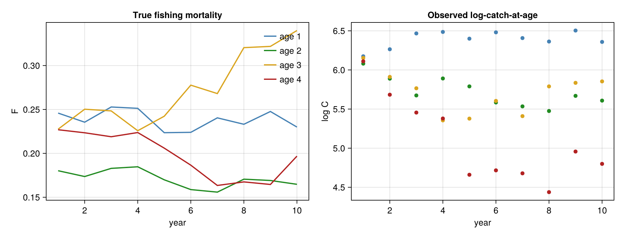
The @latte model
The model reads like the generative process above. Latent age-year fields are declared as matrices and indexed logN[a, y] — the natural notation for a state-space assessment. @latte reads the ~ statements, recognises that logN and logF form one coupled latent field, and detects the exp(logF) nonlinearity.
@latte function sam(logC, nA, nY)
    log_σN ~ Normal(-2.0, 0.5)
    log_σF ~ Normal(-2.0, 0.5)
    log_σc ~ Normal(-2.0, 0.5)
    σN = exp(log_σN)
    σF = exp(log_σF)
    σc = exp(log_σc)
    M = 0.2

    logN = Matrix{Real}(undef, nA, nY)
    logF = Matrix{Real}(undef, nA, nY)

    # Year 1: weakly informative priors on the initial age structure.
    for a in 1:nA
        logN[a, 1] ~ Normal(8.0, 0.5)
        logF[a, 1] ~ Normal(-1.5, 0.5)
    end

    # Process dynamics for the remaining years.
    for y in 2:nY
        for a in 1:nA
            logF[a, y] ~ Normal(logF[a, y - 1], σF)          # F random walk in time
        end
        logN[1, y] ~ Normal(logN[1, y - 1], σN)              # recruitment random walk
        for a in 2:nA                                        # survival (nonlinear in logF)
            logN[a, y] ~ Normal(logN[a - 1, y - 1] - exp(logF[a - 1, y - 1]) - M, σN)
        end
    end

    # Baranov catch-at-age likelihood.
    for y in 1:nY, a in 1:nA
        Z = exp(logF[a, y]) + M
        predC = logN[a, y] + logF[a, y] - log(Z) + log1p(-exp(-Z))
        logC[(y - 1) * nA + a] ~ Normal(predC, σc)
    end
end
sam (generic function with 1 method)Building the model surfaces the recognition: the latent prior is a NonGaussianLatentPrior over the stacked [logN; logF] field, 2 · nA · nY = 80 dimensions.
lgm = sam(logC, nA, nY)
lgm.latent_prior
StructuredLatentPrior{Tuple{GaussianMarkovRandomFields.LatentFactorGroup{1, Main.var"##277".var"#__latte_sprior_builder_sam##0#__latte_sprior_builder_sam##1"}, GaussianMarkovRandomFields.LatentFactorGroup{1, Main.var"##277".var"#__latte_sprior_builder_sam##2#__latte_sprior_builder_sam##3"}, GaussianMarkovRandomFields.LatentFactorGroup{2, Main.var"##277".var"#__latte_sprior_builder_sam##4#__latte_sprior_builder_sam##5"}, GaussianMarkovRandomFields.LatentFactorGroup{2, Main.var"##277".var"#__latte_sprior_builder_sam##6#__latte_sprior_builder_sam##7"}, GaussianMarkovRandomFields.LatentFactorGroup{3, Main.var"##277".var"#__latte_sprior_builder_sam##8#__latte_sprior_builder_sam##9"}}, Tuple{Vector{Tuple{Tuple{Int64}}}, Vector{Tuple{Tuple{Int64}}}, Vector{Tuple{Tuple{Int64, Int64}, Tuple{Int64, Int64}}}, Vector{Tuple{Tuple{Int64, Int64}, Tuple{Int64, Int64}}}, Vector{Tuple{Tuple{Int64, Int64, Int64}, Tuple{Int64, Int64, Int64}, Tuple{Int64, Int64, Int64}}}}, Tuple{Symbol, Symbol, Symbol}, Nothing}(80, (GaussianMarkovRandomFields.LatentFactorGroup{1, Main.var"##277".var"#__latte_sprior_builder_sam##0#__latte_sprior_builder_sam##1"}([(1,), (2,), (3,), (4,)], Main.var"##277".var"#__latte_sprior_builder_sam##0#__latte_sprior_builder_sam##1"()), GaussianMarkovRandomFields.LatentFactorGroup{1, Main.var"##277".var"#__latte_sprior_builder_sam##2#__latte_sprior_builder_sam##3"}([(41,), (42,), (43,), (44,)], Main.var"##277".var"#__latte_sprior_builder_sam##2#__latte_sprior_builder_sam##3"()), GaussianMarkovRandomFields.LatentFactorGroup{2, Main.var"##277".var"#__latte_sprior_builder_sam##4#__latte_sprior_builder_sam##5"}([(45, 41), (46, 42), (47, 43), (48, 44), (49, 45), (50, 46), (51, 47), (52, 48), (53, 49), (54, 50), (55, 51), (56, 52), (57, 53), (58, 54), (59, 55), (60, 56), (61, 57), (62, 58), (63, 59), (64, 60), (65, 61), (66, 62), (67, 63), (68, 64), (69, 65), (70, 66), (71, 67), (72, 68), (73, 69), (74, 70), (75, 71), (76, 72), (77, 73), (78, 74), (79, 75), (80, 76)], Main.var"##277".var"#__latte_sprior_builder_sam##4#__latte_sprior_builder_sam##5"()), GaussianMarkovRandomFields.LatentFactorGroup{2, Main.var"##277".var"#__latte_sprior_builder_sam##6#__latte_sprior_builder_sam##7"}([(5, 1), (9, 5), (13, 9), (17, 13), (21, 17), (25, 21), (29, 25), (33, 29), (37, 33)], Main.var"##277".var"#__latte_sprior_builder_sam##6#__latte_sprior_builder_sam##7"()), GaussianMarkovRandomFields.LatentFactorGroup{3, Main.var"##277".var"#__latte_sprior_builder_sam##8#__latte_sprior_builder_sam##9"}([(6, 1, 41), (7, 2, 42), (8, 3, 43), (10, 5, 45), (11, 6, 46), (12, 7, 47), (14, 9, 49), (15, 10, 50), (16, 11, 51), (18, 13, 53), (19, 14, 54), (20, 15, 55), (22, 17, 57), (23, 18, 58), (24, 19, 59), (26, 21, 61), (27, 22, 62), (28, 23, 63), (30, 25, 65), (31, 26, 66), (32, 27, 67), (34, 29, 69), (35, 30, 70), (36, 31, 71), (38, 33, 73), (39, 34, 74), (40, 35, 75)], Main.var"##277".var"#__latte_sprior_builder_sam##8#__latte_sprior_builder_sam##9"())), sparse([1, 5, 6, 41, 2, 7, 42, 3, 8, 43, 4, 44, 1, 5, 9, 10, 45, 1, 6, 11, 41, 46, 2, 7, 12, 42, 47, 3, 8, 43, 48, 5, 9, 13, 14, 49, 5, 10, 15, 45, 50, 6, 11, 16, 46, 51, 7, 12, 47, 52, 9, 13, 17, 18, 53, 9, 14, 19, 49, 54, 10, 15, 20, 50, 55, 11, 16, 51, 56, 13, 17, 21, 22, 57, 13, 18, 23, 53, 58, 14, 19, 24, 54, 59, 15, 20, 55, 60, 17, 21, 25, 26, 61, 17, 22, 27, 57, 62, 18, 23, 28, 58, 63, 19, 24, 59, 64, 21, 25, 29, 30, 65, 21, 26, 31, 61, 66, 22, 27, 32, 62, 67, 23, 28, 63, 68, 25, 29, 33, 34, 69, 25, 30, 35, 65, 70, 26, 31, 36, 66, 71, 27, 32, 67, 72, 29, 33, 37, 38, 73, 29, 34, 39, 69, 74, 30, 35, 40, 70, 75, 31, 36, 71, 76, 33, 37, 77, 33, 38, 73, 78, 34, 39, 74, 79, 35, 40, 75, 80, 1, 6, 41, 45, 2, 7, 42, 46, 3, 8, 43, 47, 4, 44, 48, 5, 10, 41, 45, 49, 6, 11, 42, 46, 50, 7, 12, 43, 47, 51, 8, 44, 48, 52, 9, 14, 45, 49, 53, 10, 15, 46, 50, 54, 11, 16, 47, 51, 55, 12, 48, 52, 56, 13, 18, 49, 53, 57, 14, 19, 50, 54, 58, 15, 20, 51, 55, 59, 16, 52, 56, 60, 17, 22, 53, 57, 61, 18, 23, 54, 58, 62, 19, 24, 55, 59, 63, 20, 56, 60, 64, 21, 26, 57, 61, 65, 22, 27, 58, 62, 66, 23, 28, 59, 63, 67, 24, 60, 64, 68, 25, 30, 61, 65, 69, 26, 31, 62, 66, 70, 27, 32, 63, 67, 71, 28, 64, 68, 72, 29, 34, 65, 69, 73, 30, 35, 66, 70, 74, 31, 36, 67, 71, 75, 32, 68, 72, 76, 33, 38, 69, 73, 77, 34, 39, 70, 74, 78, 35, 40, 71, 75, 79, 36, 72, 76, 80, 37, 73, 77, 38, 74, 78, 39, 75, 79, 40, 76, 80], [1, 1, 1, 1, 2, 2, 2, 3, 3, 3, 4, 4, 5, 5, 5, 5, 5, 6, 6, 6, 6, 6, 7, 7, 7, 7, 7, 8, 8, 8, 8, 9, 9, 9, 9, 9, 10, 10, 10, 10, 10, 11, 11, 11, 11, 11, 12, 12, 12, 12, 13, 13, 13, 13, 13, 14, 14, 14, 14, 14, 15, 15, 15, 15, 15, 16, 16, 16, 16, 17, 17, 17, 17, 17, 18, 18, 18, 18, 18, 19, 19, 19, 19, 19, 20, 20, 20, 20, 21, 21, 21, 21, 21, 22, 22, 22, 22, 22, 23, 23, 23, 23, 23, 24, 24, 24, 24, 25, 25, 25, 25, 25, 26, 26, 26, 26, 26, 27, 27, 27, 27, 27, 28, 28, 28, 28, 29, 29, 29, 29, 29, 30, 30, 30, 30, 30, 31, 31, 31, 31, 31, 32, 32, 32, 32, 33, 33, 33, 33, 33, 34, 34, 34, 34, 34, 35, 35, 35, 35, 35, 36, 36, 36, 36, 37, 37, 37, 38, 38, 38, 38, 39, 39, 39, 39, 40, 40, 40, 40, 41, 41, 41, 41, 42, 42, 42, 42, 43, 43, 43, 43, 44, 44, 44, 45, 45, 45, 45, 45, 46, 46, 46, 46, 46, 47, 47, 47, 47, 47, 48, 48, 48, 48, 49, 49, 49, 49, 49, 50, 50, 50, 50, 50, 51, 51, 51, 51, 51, 52, 52, 52, 52, 53, 53, 53, 53, 53, 54, 54, 54, 54, 54, 55, 55, 55, 55, 55, 56, 56, 56, 56, 57, 57, 57, 57, 57, 58, 58, 58, 58, 58, 59, 59, 59, 59, 59, 60, 60, 60, 60, 61, 61, 61, 61, 61, 62, 62, 62, 62, 62, 63, 63, 63, 63, 63, 64, 64, 64, 64, 65, 65, 65, 65, 65, 66, 66, 66, 66, 66, 67, 67, 67, 67, 67, 68, 68, 68, 68, 69, 69, 69, 69, 69, 70, 70, 70, 70, 70, 71, 71, 71, 71, 71, 72, 72, 72, 72, 73, 73, 73, 73, 73, 74, 74, 74, 74, 74, 75, 75, 75, 75, 75, 76, 76, 76, 76, 77, 77, 77, 78, 78, 78, 79, 79, 79, 80, 80, 80], Bool[1, 1, 1, 1, 1, 1, 1, 1, 1, 1, 1, 1, 1, 1, 1, 1, 1, 1, 1, 1, 1, 1, 1, 1, 1, 1, 1, 1, 1, 1, 1, 1, 1, 1, 1, 1, 1, 1, 1, 1, 1, 1, 1, 1, 1, 1, 1, 1, 1, 1, 1, 1, 1, 1, 1, 1, 1, 1, 1, 1, 1, 1, 1, 1, 1, 1, 1, 1, 1, 1, 1, 1, 1, 1, 1, 1, 1, 1, 1, 1, 1, 1, 1, 1, 1, 1, 1, 1, 1, 1, 1, 1, 1, 1, 1, 1, 1, 1, 1, 1, 1, 1, 1, 1, 1, 1, 1, 1, 1, 1, 1, 1, 1, 1, 1, 1, 1, 1, 1, 1, 1, 1, 1, 1, 1, 1, 1, 1, 1, 1, 1, 1, 1, 1, 1, 1, 1, 1, 1, 1, 1, 1, 1, 1, 1, 1, 1, 1, 1, 1, 1, 1, 1, 1, 1, 1, 1, 1, 1, 1, 1, 1, 1, 1, 1, 1, 1, 1, 1, 1, 1, 1, 1, 1, 1, 1, 1, 1, 1, 1, 1, 1, 1, 1, 1, 1, 1, 1, 1, 1, 1, 1, 1, 1, 1, 1, 1, 1, 1, 1, 1, 1, 1, 1, 1, 1, 1, 1, 1, 1, 1, 1, 1, 1, 1, 1, 1, 1, 1, 1, 1, 1, 1, 1, 1, 1, 1, 1, 1, 1, 1, 1, 1, 1, 1, 1, 1, 1, 1, 1, 1, 1, 1, 1, 1, 1, 1, 1, 1, 1, 1, 1, 1, 1, 1, 1, 1, 1, 1, 1, 1, 1, 1, 1, 1, 1, 1, 1, 1, 1, 1, 1, 1, 1, 1, 1, 1, 1, 1, 1, 1, 1, 1, 1, 1, 1, 1, 1, 1, 1, 1, 1, 1, 1, 1, 1, 1, 1, 1, 1, 1, 1, 1, 1, 1, 1, 1, 1, 1, 1, 1, 1, 1, 1, 1, 1, 1, 1, 1, 1, 1, 1, 1, 1, 1, 1, 1, 1, 1, 1, 1, 1, 1, 1, 1, 1, 1, 1, 1, 1, 1, 1, 1, 1, 1, 1, 1, 1, 1, 1, 1, 1, 1, 1, 1, 1, 1, 1], 80, 80), ([((1,),), ((5,),), ((8,),), ((11,),)], [((182,),), ((186,),), ((190,),), ((193,),)], [((198, 183), (197, 182)), ((203, 187), (202, 186)), ((208, 191), (207, 190)), ((212, 194), (211, 193)), ((217, 199), (216, 198)), ((222, 204), (221, 203)), ((227, 209), (226, 208)), ((231, 213), (230, 212)), ((236, 218), (235, 217)), ((241, 223), (240, 222)), ((246, 228), (245, 227)), ((250, 232), (249, 231)), ((255, 237), (254, 236)), ((260, 242), (259, 241)), ((265, 247), (264, 246)), ((269, 251), (268, 250)), ((274, 256), (273, 255)), ((279, 261), (278, 260)), ((284, 266), (283, 265)), ((288, 270), (287, 269)), ((293, 275), (292, 274)), ((298, 280), (297, 279)), ((303, 285), (302, 284)), ((307, 289), (306, 288)), ((312, 294), (311, 293)), ((317, 299), (316, 298)), ((322, 304), (321, 303)), ((326, 308), (325, 307)), ((331, 313), (330, 312)), ((336, 318), (335, 317)), ((341, 323), (340, 322)), ((345, 327), (344, 326)), ((349, 332), (348, 331)), ((352, 337), (351, 336)), ((355, 342), (354, 341)), ((358, 346), (357, 345))], [((14, 2), (13, 1)), ((33, 15), (32, 14)), ((52, 34), (51, 33)), ((71, 53), (70, 52)), ((90, 72), (89, 71)), ((109, 91), (108, 90)), ((128, 110), (127, 109)), ((147, 129), (146, 128)), ((166, 148), (165, 147))], [((19, 3, 181), (18, 1, 180), (21, 4, 182)), ((24, 6, 185), (23, 5, 184), (26, 7, 186)), ((29, 9, 189), (28, 8, 188), (30, 10, 190)), ((38, 16, 196), (37, 14, 195), (40, 17, 198)), ((43, 20, 201), (42, 19, 200), (45, 22, 203)), ((48, 25, 206), (47, 24, 205), (49, 27, 208)), ((57, 35, 215), (56, 33, 214), (59, 36, 217)), ((62, 39, 220), (61, 38, 219), (64, 41, 222)), ((67, 44, 225), (66, 43, 224), (68, 46, 227)), ((76, 54, 234), (75, 52, 233), (78, 55, 236)), ((81, 58, 239), (80, 57, 238), (83, 60, 241)), ((86, 63, 244), (85, 62, 243), (87, 65, 246)), ((95, 73, 253), (94, 71, 252), (97, 74, 255)), ((100, 77, 258), (99, 76, 257), (102, 79, 260)), ((105, 82, 263), (104, 81, 262), (106, 84, 265)), ((114, 92, 272), (113, 90, 271), (116, 93, 274)), ((119, 96, 277), (118, 95, 276), (121, 98, 279)), ((124, 101, 282), (123, 100, 281), (125, 103, 284)), ((133, 111, 291), (132, 109, 290), (135, 112, 293)), ((138, 115, 296), (137, 114, 295), (140, 117, 298)), ((143, 120, 301), (142, 119, 300), (144, 122, 303)), ((152, 130, 310), (151, 128, 309), (154, 131, 312)), ((157, 134, 315), (156, 133, 314), (159, 136, 317)), ((162, 139, 320), (161, 138, 319), (163, 141, 322)), ((169, 149, 329), (168, 147, 328), (170, 150, 331)), ((173, 153, 334), (172, 152, 333), (174, 155, 336)), ((177, 158, 339), (176, 157, 338), (178, 160, 341))]), (:log_σN, :log_σF, :log_σc), :structured, nothing)Inference
inla explores the three-dimensional hyperparameter posterior and integrates the latent field out at each point with an iterated Laplace approximation — re-linearising the nonlinear survival recursion at every Newton step rather than once. We keep the marginal log-likelihood accumulator for model comparison and skip the pointwise predictive metrics, which fall back to Monte Carlo for the nonlinear catch likelihood.
result = inla(lgm, logC; progress = false, accumulators = (MarginalLogLikelihoodStrategy(),))INLAResult:
Model: LatentGaussianModel{HyperparameterSpec{@NamedTuple{log_σN::Hyperparameter{typeof(identity), :natural}, log_σF::Hyperparameter{typeof(identity), :natural}, log_σc::Hyperparameter{typeof(identity), :natural}}, @NamedTuple{}}, StructuredLatentPrior{Tuple{GaussianMarkovRandomFields.LatentFactorGroup{1, Main.var"##277".var"#__latte_sprior_builder_sam##0#__latte_sprior_builder_sam##1"}, GaussianMarkovRandomFields.LatentFactorGroup{1, Main.var"##277".var"#__latte_sprior_builder_sam##2#__latte_sprior_builder_sam##3"}, GaussianMarkovRandomFields.LatentFactorGroup{2, Main.var"##277".var"#__latte_sprior_builder_sam##4#__latte_sprior_builder_sam##5"}, GaussianMarkovRandomFields.LatentFactorGroup{2, Main.var"##277".var"#__latte_sprior_builder_sam##6#__latte_sprior_builder_sam##7"}, GaussianMarkovRandomFields.LatentFactorGroup{3, Main.var"##277".var"#__latte_sprior_builder_sam##8#__latte_sprior_builder_sam##9"}}, Tuple{Vector{Tuple{Tuple{Int64}}}, Vector{Tuple{Tuple{Int64}}}, Vector{Tuple{Tuple{Int64, Int64}, Tuple{Int64, Int64}}}, Vector{Tuple{Tuple{Int64, Int64}, Tuple{Int64, Int64}}}, Vector{Tuple{Tuple{Int64, Int64, Int64}, Tuple{Int64, Int64, Int64}, Tuple{Int64, Int64, Int64}}}}, Tuple{Symbol, Symbol, Symbol}, Nothing}, GaussianMarkovRandomFields.StructuredObservationModel{Tuple{GaussianMarkovRandomFields.ObsFactorGroup{2, Main.var"##277".var"#__latte_sobs_builder_sam##0#__latte_sobs_builder_sam##1"}}, Tuple{Symbol}}}
Hyperparameters: 3
Latent variables: 80
Mode: (log_σN=-2.396, log_σF=-2.2837, log_σc=-2.7392)
Convergence: ✓
Total time: 39.57 seconds
Exploration: 15 points (15 integration)
Model comparison metrics:
Marginal Log-Likelihood:
log p(y): 0.29
Use .hyperparameter_marginals, .latent_marginals, .accumulators for analysisA note Latte prints on the first call: a non-Gaussian latent prior is reported through Gaussian marginals. The posterior mean and precision from the iterated Laplace are exact; only the higher-moment skew of each marginal is not yet corrected for non-Gaussian priors. For the smooth fields here that is a small effect.
Recovering the latent field
The posterior means reshape back to the age-year grid. Both fields are recovered closely despite only catch being observed:
mN = reshape(mean.(latent_marginals(result, :logN)), nA, nY)
mF = reshape(mean.(latent_marginals(result, :logF)), nA, nY)
sF = reshape(std.(latent_marginals(result, :logF)), nA, nY)

(logN_maxerr = maximum(abs.(mN .- logN_t)), logF_maxerr = maximum(abs.(mF .- logF_t)))
(logN_maxerr = 0.19469611693840427, logF_maxerr = 0.20348768829700625)Fishing mortality per age, with the posterior mean, a 95% credible band, and the truth. The latent field tracks the simulated dynamics across all four ages:
fig2 = Figure(size = (1000, 640))
for a in 1:nA
    row, col = fldmod1(a, 2)
    ax = Axis(fig2[row, col], title = "log F — age $a", xlabel = "year", ylabel = "log F")
    band!(
        ax, 1:nY, mF[a, :] .- 1.96 .* sF[a, :], mF[a, :] .+ 1.96 .* sF[a, :];
        color = (:steelblue, 0.25),
    )
    lines!(ax, 1:nY, mF[a, :]; color = :steelblue, linewidth = 2, label = "posterior mean")
    lines!(ax, 1:nY, logF_t[a, :]; color = :black, linestyle = :dash, label = "truth")
    a == 1 && axislegend(ax; position = :rb, framevisible = false)
end
fig2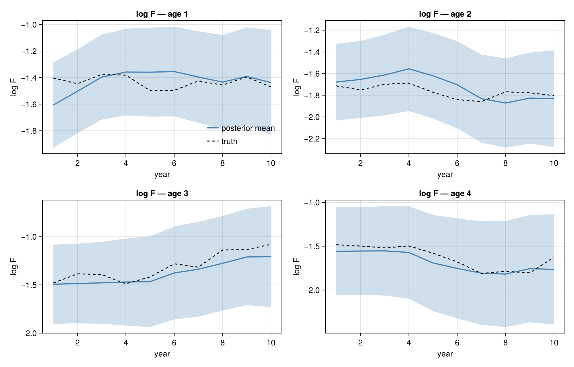
The hyperparameter posterior
The three standard deviations are reported on their natural scale. Each was declared on the log scale, so the natural-scale point estimate is the exponential of the marginal's median:
using DataFrames

hp_keys = collect(keys(lgm.hyperparameter_spec.free))
truth = (σN = σN_true, σF = σF_true, σc = σc_true)
summary_hp = DataFrame(
    parameter = [Symbol(string(k)[5:end]) for k in hp_keys],
    truth = [getproperty(truth, Symbol(string(k)[5:end])) for k in hp_keys],
    posterior_median = [exp(median(hyperparameter_marginals(result, k)[1])) for k in hp_keys],
)
3×3 DataFrame
Row │ parameter truth posterior_median
│ Symbol Float64 Float64
─────┼──────────────────────────────────────
1 │ σN 0.1 0.0917154
2 │ σF 0.1 0.101816
3 │ σc 0.1 0.0632145Management quantities
Assessments are run to inform management, and the quantities managers act on — spawning-stock biomass (SSB) and the average fishing mortality on the exploited ages (Fbar) — are nonlinear functions of the latent field. derived pushes posterior draws through any such function and returns its full marginal, so these summaries carry the posterior uncertainty of the latent field rather than a single plug-in value. It is the sampling-based, nonlinear counterpart to linear_combinations.
SSB weights numbers-at-age by weight and maturity; Fbar averages F over a reference age range (here ages 2–4). The closure receives one posterior draw as a NamedTuple of the latent groups; we reshape each flattened field back to age × year and return one value per year:
weight_at_age = [0.1, 0.4, 0.9, 1.5]      # illustrative weight-at-age
maturity_at_age = [0.0, 0.5, 1.0, 1.0]    # proportion mature at age

ssb = derived(result; n_samples = 2000) do z
    logN = reshape(z.logN, nA, nY)
    [sum(weight_at_age .* maturity_at_age .* exp.(logN[:, y])) for y in 1:nY]
end
fbar = derived(result; n_samples = 2000) do z
    logF = reshape(z.logF, nA, nY)
    [mean(exp.(logF[2:nA, y])) for y in 1:nY]
end
10-element Vector{SampleMarginal{Float64}}:
SampleMarginal(n=2000, mean=0.2125, std=0.0435)
SampleMarginal(n=2000, mean=0.2152, std=0.0454)
SampleMarginal(n=2000, mean=0.219, std=0.0487)
SampleMarginal(n=2000, mean=0.2228, std=0.0517)
SampleMarginal(n=2000, mean=0.2109, std=0.051)
SampleMarginal(n=2000, mean=0.2094, std=0.052)
SampleMarginal(n=2000, mean=0.2023, std=0.0512)
SampleMarginal(n=2000, mean=0.2056, std=0.0524)
SampleMarginal(n=2000, mean=0.2191, std=0.0575)
SampleMarginal(n=2000, mean=0.2191, std=0.0592)Each entry of ssb and fbar is a SampleMarginal, so mean, std, and quantile work directly. Against the truth, with 95% credible bands:
ssb_true = [sum(weight_at_age .* maturity_at_age .* exp.(logN_t[:, y])) for y in 1:nY]
fbar_true = [mean(exp.(logF_t[2:nA, y])) for y in 1:nY]

fig3 = Figure(size = (1000, 380))
ax_ssb = Axis(fig3[1, 1], title = "Spawning-stock biomass", xlabel = "year", ylabel = "SSB")
ax_fbar = Axis(fig3[1, 2], title = "Average F (ages 2–4)", xlabel = "year", ylabel = "Fbar")
for (ax, q, qt) in ((ax_ssb, ssb, ssb_true), (ax_fbar, fbar, fbar_true))
    band!(ax, 1:nY, [quantile(qi, 0.025) for qi in q], [quantile(qi, 0.975) for qi in q]; color = (:steelblue, 0.25))
    lines!(ax, 1:nY, mean.(q); color = :steelblue, linewidth = 2, label = "posterior mean")
    lines!(ax, 1:nY, qt; color = :black, linestyle = :dash, label = "truth")
end
axislegend(ax_ssb; position = :rt, framevisible = false)
fig3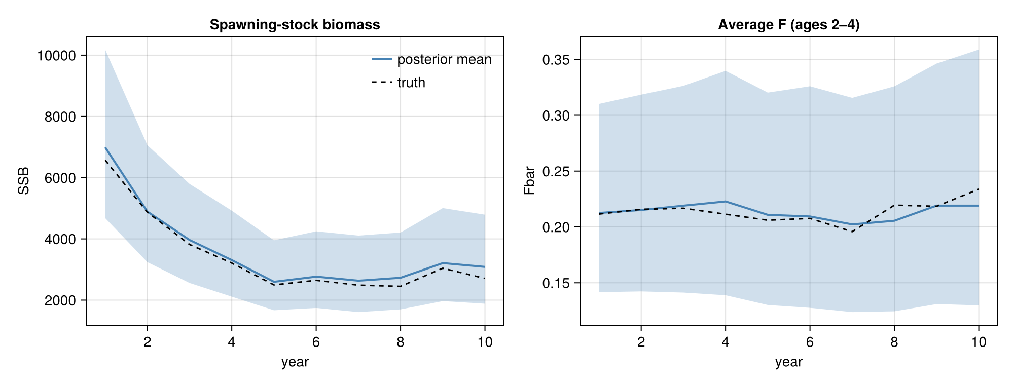
The same model through tmb
Swapping the engine needs no change to the model. tmb finds the hyperparameter MAP, takes the outer Hessian for standard errors, and reconstructs the inner Laplace at the MAP — the workflow most age-structured assessments use in practice. Its latent reconstruction matches inla's to plotting precision:
result_tmb = tmb(lgm, logC)
mF_tmb = reshape(mean.(latent_marginals(result_tmb, :logF)), nA, nY)

(inla_vs_tmb_maxdiff = maximum(abs.(mF .- mF_tmb)),)
(inla_vs_tmb_maxdiff = 0.008581402481895095,)Validation against NUTS
Both engines are Laplace approximations, so agreeing with each other is reassuring but not conclusive. To check the approximation itself we sample the same model with NUTS — full Hamiltonian Monte Carlo, no Gaussian approximation anywhere — through the @latte → DynamicPPL handoff. Latte.dppl_model returns the underlying generative model, which Turing samples directly.
using Turing

dppl = Latte.dppl_model(sam)(logC, nA, nY)
nuts_chain = sample(dppl, NUTS(500, 0.8), 1000; progress = false)
mN_nuts = reshape([mean(nuts_chain[Symbol("logN[$a, $y]")]) for y in 1:nY for a in 1:nA], nA, nY)
mF_nuts = reshape([mean(nuts_chain[Symbol("logF[$a, $y]")]) for y in 1:nY for a in 1:nA], nA, nY)

(logN_max_abs_diff = maximum(abs.(mN .- mN_nuts)), logF_max_abs_diff = maximum(abs.(mF .- mF_nuts)))
(logN_max_abs_diff = 0.050846964329695155, logF_max_abs_diff = 0.05969281291691053)The iterated-Laplace posterior means match the MCMC gold standard across the whole latent field, to within Monte Carlo error. The left panel plots every cell's posterior mean, INLA against NUTS, on the y = x line; the right panel overlays the full INLA marginal for one fishing-mortality cell on the NUTS samples.
mF_marg = reshape(latent_marginals(result, :logF), nA, nY)
m = mF_marg[2, nY]
fcell = vec(Array(nuts_chain[Symbol("logF[2, $nY]")]))

fig4 = Figure(size = (1000, 380))
ax_s = Axis(fig4[1, 1], title = "Posterior means: INLA vs NUTS", xlabel = "NUTS", ylabel = "INLA")
ablines!(ax_s, 0, 1; color = :black, linestyle = :dash)
scatter!(ax_s, vec(mN_nuts), vec(mN); color = (:steelblue, 0.6), label = "log N")
scatter!(ax_s, vec(mF_nuts), vec(mF); color = (:firebrick, 0.6), label = "log F")
axislegend(ax_s; position = :lt, framevisible = false)

ax_m = Axis(fig4[1, 2], title = "Marginal: log F (age 2, year $nY)", xlabel = "log F", ylabel = "density")
hist!(ax_m, fcell; normalization = :pdf, bins = 30, color = (:firebrick, 0.3), label = "NUTS")
xs = range(minimum(fcell), maximum(fcell); length = 100)
lines!(ax_m, xs, pdf.(Normal(mean(m), std(m)), xs); color = :steelblue, linewidth = 2, label = "INLA")
axislegend(ax_m; position = :rt, framevisible = false)
fig4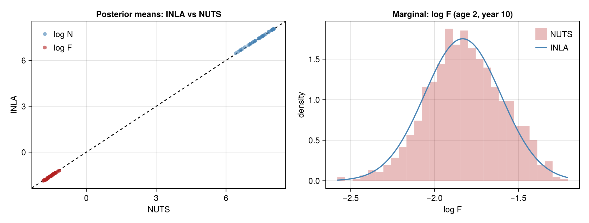
What this demonstrates
The nonlinear survival recursion makes the latent prior non-Gaussian, and @latte handles it from the model definition alone: it recognises that logN and logF form one coupled field, detects the exp(logF) curvature, and routes the fit to an iterated Laplace approximation. The same sam model runs unchanged through inla (full hyperparameter posterior) and tmb (MAP with standard errors), so the choice of engine is a runtime decision, not a modelling one. The NUTS comparison above is the check that matters: the approximation reproduces the full-MCMC posterior across the latent field.
The age-year latent fields are written with natural matrix indexing, logN[a, y], rather than hand-flattened vectors, and the sparse structure of the survival recursion is exploited automatically — the per-iterate factorisation stays banded and the cost grows linearly in the number of years.
A few directions to extend this:
A plus group at the oldest age, where survivors accumulate rather than age out.
Selectivity-at-age, separating
F_{a, y}into a year effect and an age-selectivity curve, as in the original SAM formulation.A second observation series, such as a research survey index, added as one more
~block with its own catchability and noise, to anchor absolute stock size.Reference points (MSY, F_MSY, B_MSY) and short-term forecasts, both further
derivedquantities built on the SSB and Fbar marginals above.
For the inference protocol shared across inla, tmb, and hmc_laplace, see the API reference.
References
The state-space assessment model (SAM): numbers-at-age and fishing mortality as coupled latent random walks, integrated out by a Laplace approximation.
Standard reference for age-structured population dynamics, including the Baranov catch equation relating catch to numbers-at-age and instantaneous mortality rates.
This page was generated using Literate.jl.