Bayesian Model Averaging

When several candidate models are on the table, committing to a single one discards whatever the others have to say. Bayesian model averaging (BMA) keeps all of them, combining their posterior marginals with weights set by how well each explains the data, so the final inference carries the uncertainty about which model is right (Hoeting et al., 1999).

Given $K$ models $M_{1}, \dots, M_{K}$ , the averaged posterior for a quantity of interest is

p (Δ ∣ y) = \sum_{k = 1}^{K} p (Δ ∣ y, M_{k}) \cdot p (M_{k} ∣ y)

where the model weights are $p (M_{k} ∣ y) \propto p (y ∣ M_{k}) \cdot p (M_{k})$ . The marginal likelihood $p (y ∣ M_{k})$ is a by-product of the INLA fit, so the weights cost nothing extra once the individual models are in hand.

Averaging is only interesting when no single model dominates. If one model has a far larger marginal likelihood than the rest, its weight collapses to one and the average reduces to that model. The useful case is several models with comparable support, where the data genuinely cannot decide between them. This tutorial works through such a case: two competing smoothness structures for a time series whose marginal likelihoods come out nearly tied.

The dataset: global earthquake activity

We reuse the annual counts of major earthquakes (magnitude $\geq 7$ ) from 1900 to 2006 introduced in the temporal trend tutorial. The data come from Zucchini et al. (2016); with 107 observations they fit in a single block:

julia

using DataFrames
quake_counts = [
    13, 14, 8, 10, 16, 26, 32, 27, 18, 32, 36, 24, 20, 23, 23, 18, 12,
    20, 22, 19, 13, 26, 13, 14, 22, 24, 21, 22, 26, 21, 23, 24, 20, 24, 24, 22,
    20, 10, 14, 19, 23, 18, 12, 13, 20, 26, 35, 14, 17, 19, 15, 18, 22, 22, 17,
    22, 15, 34, 10, 15, 22, 18, 15, 20, 13, 22, 23, 15, 21, 19, 20, 11, 20, 13,
    10, 8, 15, 18, 15, 9, 13, 13, 14, 9, 13, 16, 15, 8, 5, 11, 13, 7, 15, 12, 23,
    25, 22, 21, 20, 16, 14, 15, 13, 14, 17, 14, 11,
]
eq_data = DataFrame(year = 1900:2006, quakes = quake_counts)
n_years = nrow(eq_data)
first(eq_data, 5)

5×2 DataFrame
 Row │ year   quakes
     │ Int64  Int64
─────┼───────────────
   1 │  1900      13
   2 │  1901      14
   3 │  1902       8
   4 │  1903      10
   5 │  1904      16

Two competing trend models

We model the annual count $y_{t}$ as Poisson with a log-rate built from an intercept and a latent temporal effect $f_{t}$ :

y_{t} \sim Poisson (λ_{t}), \log λ_{t} = β_{0} + f_{t} .

The two models differ only in the prior on $f$ , i.e. in what kind of trend they expect. Both place a latent effect of the same length on the same years, so their latent fields line up position by position — exactly what averaging needs.

Model A — first-order random walk (RW1). The first differences of $f$ are i.i.d. Gaussian, penalising abrupt jumps in level. This gives a locally adaptive trend that can change direction cheaply from year to year.

Model B — first-order autoregression (AR1). Here $f$ mean-reverts toward zero with correlation $ρ$ between neighbouring years, $f_{t} = ρ f_{t - 1} + ε_{t}$ . Instead of a free-floating walk, deviations decay back to the overall level.

Both priors come from GaussianMarkovRandomFields.jl, called inside @latte so the macro recognizes them as structured Gaussians.

julia

using Latte
using Distributions
using GaussianMarkovRandomFields: RWModel, AR1Model
using LinearAlgebra

@latte function quake_rw1(y, n)
    τ_rw ~ PCPrior.Precision(1.0, α = 0.01)
    β ~ MvNormal(zeros(1), 100.0 * I(1))
    f ~ RWModel{1}(n)(τ = τ_rw)
    for i in eachindex(y)
        y[i] ~ Poisson(exp(β[1] + f[i]))
    end
end

@latte function quake_ar1(y, n)
    τ_ar ~ PCPrior.Precision(1.0, α = 0.01)
    ρ ~ Uniform(-1.0, 1.0)
    β ~ MvNormal(zeros(1), 100.0 * I(1))
    f ~ AR1Model(n)(τ = τ_ar, ρ = ρ)
    for i in eachindex(y)
        y[i] ~ Poisson(exp(β[1] + f[i]))
    end
end

quake_ar1 (generic function with 1 method)

The precision prior PCPrior.Precision(1.0, α = 0.01) is a penalised-complexity prior (Simpson et al., 2017): it says "there is only a 1% chance the standard deviation of the innovations exceeds 1", shrinking each model toward a flat trend unless the data pull it away. We give both models the same precision prior so the comparison turns on trend structure, not on prior scale.

Calling each @latte function builds a LatentGaussianModel; inla runs on it.

julia

lgm_rw1 = quake_rw1(eq_data.quakes, n_years)
result_rw1 = inla(lgm_rw1, eq_data.quakes; progress = false)

lgm_ar1 = quake_ar1(eq_data.quakes, n_years)
result_ar1 = inla(lgm_ar1, eq_data.quakes; progress = false)

INLAResult:
  Model: LatentGaussianModel{HyperparameterSpec{@NamedTuple{τ_ar::Hyperparameter{Bijectors.TruncatedBijector{Float64, Float64}, :natural}, ρ::Hyperparameter{Bijectors.TruncatedBijector{Float64, Float64}, :natural}}, @NamedTuple{}}, Latte._PatternAugmentedLatentModel{Latte.RoutedLatentModel{CombinedModel{LinearSolve.CHOLMODFactorization{Nothing}}, @NamedTuple{τ_ar1::Symbol, ρ_ar1::Symbol}}, SparseArrays.SparseMatrixCSC{Int64, Int64}}, LinearlyTransformedObservationModel{ExponentialFamily{Distributions.Poisson, LogLink, Nothing, Nothing}, SparseArrays.SparseMatrixCSC{Float64, Int64}, Nothing}}
  Hyperparameters: 2
  Latent variables: 108
  Mode: (τ_ar=38.5361, ρ=0.7802)
  Convergence: ✓
  Total time: 13.96 seconds
  Exploration: 17 points (17 integration)

Model comparison metrics:
Deviance Information Criterion (DIC):
  DIC: 573.07
  Effective parameters (p_D): 3.19
  Mean deviance (D̄): 569.87
  Deviance at mode: 566.68

Marginal Log-Likelihood:
  log p(y): -338.81

Watanabe-Akaike Information Criterion (WAIC):
  WAIC: 627.4
  Effective parameters (p_WAIC): 22.14
  Log pointwise predictive density (lppd): -291.56

Conditional Predictive Ordinates (CPO):
  LPML: -311.63
  Mean CPO: 0.0631
  Min CPO: 0.0006
  PIT computed: 107 values
  PIT mean: 0.4918 (ideal: 0.5)


Approximation quality (KLD):
  Max SKLD: 0.0086 (variable 1)
  Mean SKLD: 0.0016

Use .hyperparameter_marginals, .latent_marginals, .accumulators for analysis

Comparing marginal likelihoods

log_marginal_likelihood(r) reads off INLA's estimate of $\log p (y ∣ M_{k})$ , the quantity the weights are built from. Larger is better-supported:

julia

log_mlls = log_marginal_likelihood.([result_rw1, result_ar1])
DataFrame(model = ["RW1", "AR1"], log_ML = round.(log_mlls, digits = 2))

2×2 DataFrame
 Row │ model   log_ML
     │ String  Float64
─────┼─────────────────
   1 │ RW1     -338.89
   2 │ AR1     -338.81

The two scores come out within a fraction of a log-unit of each other. Neither trend structure is clearly preferred: a random walk and a mean-reverting process explain this series about equally well. This is precisely the regime where averaging earns its keep.

Model averaging

model_average turns the marginal likelihoods into posterior model weights and blends the two fits position by position. It returns a BMAResult whose model_weights are the posterior model probabilities $p (M_{k} ∣ y)$ :

julia

bma = model_average([result_rw1, result_ar1])
DataFrame(model = ["RW1", "AR1"], weight = round.(bma.model_weights, digits = 3))

2×2 DataFrame
 Row │ model   weight
     │ String  Float64
─────┼─────────────────
   1 │ RW1       0.482
   2 │ AR1       0.518

The weights are split roughly evenly. The averaged posterior is therefore a real blend of both trends, not a thin veneer over one of them.

The blended trend

bma.latent_marginals holds the model-averaged marginal for each latent variable — here the intercept $β_{0}$ followed by the 107 temporal effects $f_{t}$ , each a WeightedMixture of its RW1 and AR1 counterparts. To plot a trend on the count scale we want $λ_{t} = \exp (β_{0} + f_{t})$ , which lives in the observation marginals. We blend those the same way BMA blends the latent field: a WeightedMixture of the per-year observation marginals under each model, weighted by the posterior model weights.

julia

using Latte: WeightedMixture

obs_rw1 = observation_marginals(result_rw1)
obs_ar1 = observation_marginals(result_ar1)
obs_bma = [
    WeightedMixture([obs_rw1[t], obs_ar1[t]], bma.model_weights) for t in 1:n_years
];

A tidy long-form table of the posterior-median trend for each model plus the blend lets AlgebraOfGraphics draw all three with one mapping:

julia

using AlgebraOfGraphics, CairoMakie

trend_df = vcat(
    DataFrame(year = eq_data.year, median = median.(obs_rw1), model = "RW1"),
    DataFrame(year = eq_data.year, median = median.(obs_ar1), model = "AR1"),
    DataFrame(year = eq_data.year, median = median.(obs_bma), model = "BMA"),
)
first(trend_df, 5)

5×3 DataFrame
 Row │ year   median   model
     │ Int64  Float64  String
─────┼────────────────────────
   1 │  1900  13.5857  RW1
   2 │  1901  13.6892  RW1
   3 │  1902  13.7148  RW1
   4 │  1903  15.008   RW1
   5 │  1904  17.7259  RW1

Overlaying the three medians on the raw counts:

julia

pts = data(eq_data) *
    mapping(:year => "Year", :quakes => "Major earthquakes (M ≥ 7)") *
    visual(Scatter, markersize = 5, color = :gray70)
trends = data(trend_df) *
    mapping(:year => "Year", :median => "Major earthquakes (M ≥ 7)", color = :model => "Model") *
    visual(Lines, linewidth = 2)
draw(
    pts + trends,
    axis = (title = "RW1, AR1, and the model-averaged trend",),
)

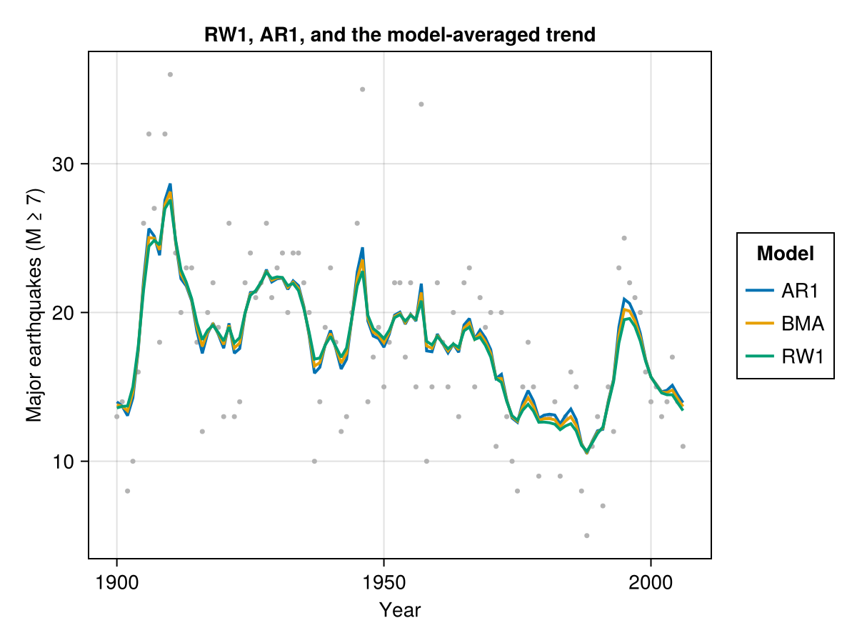
The RW1 and AR1 medians trace slightly different paths, and the BMA trend (its own colour) runs between them — closest to whichever model carries more weight at each point. Because the weights here are near 50/50, the blend sits roughly midway rather than hugging either single fit.

Uncertainty in the blend

The averaged marginal is a mixture of the two single-model marginals, so its variance is the weight-averaged variance of the two plus a term for how far apart their means sit:

{Var}_{BMA} = \sum_{k} w_{k} {Var}_{k} + \sum_{k} w_{k} (μ_{k} - \bar{μ})^{2} .

That means the blend lands between the two models' spreads, nudged upward by any disagreement in their centers — it neither copies the sharpest model nor automatically exceeds the widest. We can read this off the intercept $β_{0}$ , the first latent variable:

julia

β_bma = bma.latent_marginals[1]
β_rw1 = latent_marginals(result_rw1, :β)[1]
β_ar1 = latent_marginals(result_ar1, :β)[1]
DataFrame(
    source = ["RW1", "AR1", "BMA"],
    mean = round.(mean.([β_rw1, β_ar1, β_bma]), digits = 3),
    std = round.(std.([β_rw1, β_ar1, β_bma]), digits = 3),
)

3×3 DataFrame
 Row │ source  mean     std
     │ String  Float64  Float64
─────┼──────────────────────────
   1 │ RW1       2.857    0.024
   2 │ AR1       2.835    0.091
   3 │ BMA       2.846    0.068

The BMA standard deviation (0.068) sits between the two: well above RW1's tight 0.024 and just below AR1's 0.091, since AR1 carries slightly more weight and the two means nearly coincide. Committing to RW1 alone would have understated the intercept uncertainty almost threefold; the blend keeps the more cautious model's contribution in proportion to its support, which is the honest thing to report.

Plotting the three intercept densities shows the blend as a weighted mixture of the two. We evaluate each density on a shared grid and assemble a tidy frame for AlgebraOfGraphics:

julia

grid = range(2.4, 3.3, length = 300)
dens_df = vcat(
    DataFrame(x = grid, density = pdf.(β_rw1, grid), source = "RW1"),
    DataFrame(x = grid, density = pdf.(β_ar1, grid), source = "AR1"),
    DataFrame(x = grid, density = pdf.(β_bma, grid), source = "BMA"),
)
draw(
    data(dens_df) *
        mapping(:x => "Intercept β₀", :density => "Density", color = :source => "Source") *
        visual(Lines, linewidth = 2),
    axis = (title = "Intercept: single-model marginals vs the BMA blend",),
)

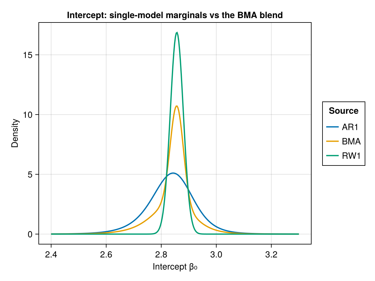
The BMA curve is a weighted mixture of the two single-model densities: it places mass over both locations in proportion to the model weights rather than collapsing onto either. Reporting it instead of a single model passes the model-selection uncertainty through to the final inference.

Using prior model weights

model_average assumes equal prior weights unless told otherwise. When prior knowledge favours one structure, pass prior_weights to tilt the comparison. Here we suppose a 3:1 prior preference for the random walk:

julia

bma_prior = model_average([result_rw1, result_ar1]; prior_weights = [0.75, 0.25])
DataFrame(model = ["RW1", "AR1"], weight = round.(bma_prior.model_weights, digits = 3))

2×2 DataFrame
 Row │ model   weight
     │ String  Float64
─────┼─────────────────
   1 │ RW1       0.736
   2 │ AR1       0.264

The prior shifts the posterior weights toward RW1, but because the marginal likelihoods are so close the data offer little to override it: the prior largely carries through.

Working with BMA results

Each averaged marginal is a WeightedMixture, so the full Distributions.jl interface applies directly. Posterior mean and a 95% credible interval for the intercept:

julia

mean(β_bma), quantile.(β_bma, (0.025, 0.975))

(2.8455136523984237, (2.681388328545836, 2.977403433055668))

summary_df tabulates the averaged latent marginals the same way it does for a single fit. We show the intercept and the first few temporal effects:

julia

first(summary_df(bma.latent_marginals), 5)

5×6 DataFrame
 Row │ mode       median     q2_5       q97_5      mean       std
     │ Float64    Float64    Float64    Float64    Float64    Float64
─────┼──────────────────────────────────────────────────────────────────
   1 │  2.85607    2.85208    2.68139   2.9774      2.84551   0.0684264
   2 │ -0.218696  -0.222133  -0.569503  0.115198   -0.223548  0.173892
   3 │ -0.225974  -0.229676  -0.54869   0.0794678  -0.231103  0.15942
   4 │ -0.24103   -0.251829  -0.586243  0.0458091  -0.256781  0.160468
   5 │ -0.151835  -0.162955  -0.487011  0.124272   -0.167979  0.154749

Summary

BMA is worthwhile when several models have comparable marginal likelihoods; a lopsided comparison just recovers the single best model.
Here a random walk and an AR1 process explain the earthquake series almost equally well, giving near-even weights and a genuine blend.
model_average reuses the marginal likelihood INLA already computes, so the weights are free once the individual fits are done.
The averaged marginals are WeightedMixture distributions: they sit between the single-model fits, with a spread that blends both models' uncertainty and their disagreement rather than committing to one model's confidence.

References

BMA

Bayesian Model Averaging: A Tutorial

J. A. Hoeting, D. Madigan, A. E. Raftery & C. T. Volinsky

Statistical Science · 1999 · doi:10.1214/ss/1009212519

The standard tutorial reference on Bayesian model averaging: combining inferences across models weighted by their posterior model probabilities to account for model uncertainty.

INLA

Approximate Bayesian Inference for Latent Gaussian Models by Using Integrated Nested Laplace Approximations

H. Rue, S. Martino & N. Chopin

J. R. Statist. Soc. B · 2009 · doi:10.1111/j.1467-9868.2008.00700.x

The original INLA paper: deterministic approximate Bayesian inference for latent Gaussian models via nested Laplace approximations and numerical integration over the hyperparameters. The marginal likelihood it reports drives the BMA weights.

PC priors

Penalising Model Component Complexity: A Principled, Practical Approach to Constructing Priors

D. Simpson, H. Rue, A. Riebler, T. G. Martins & S. H. Sørbye

Statistical Science · 2017 · doi:10.1214/16-STS576

Penalised-complexity (PC) priors: weakly informative priors that shrink a model component towards a simpler base model, used here for the random-walk and AR1 precision.

Zucchini

Hidden Markov Models for Time Series: An Introduction Using R (2nd ed.)

W. Zucchini, I. L. MacDonald & R. Langrock

Chapman & Hall/CRC · 2016 · doi:10.1201/b20790

Source of the annual major-earthquake counts (1900–2006) used here as the competing-trend example.

This page was generated using Literate.jl.

Bayesian Model Averaging ​

The dataset: global earthquake activity ​

Two competing trend models ​

Comparing marginal likelihoods ​

Model averaging ​

The blended trend ​

Uncertainty in the blend ​

Using prior model weights ​

Working with BMA results ​

Summary ​

References ​

Bayesian Model Averaging

The dataset: global earthquake activity

Two competing trend models

Comparing marginal likelihoods

Model averaging

The blended trend

Uncertainty in the blend

Using prior model weights

Working with BMA results

Summary

References