Custom likelihoods: Tweedie regression on insurance claims

A latent Gaussian model in Latte is not tied to a fixed list of observation likelihoods. Any distribution you can write down as a logpdf can go on the ~ line of an @latte model and be fit with inla(), recovering posterior marginals for the latent field and the hyperparameters together.

This tutorial works through that on the Tweedie compound Poisson-Gamma, the standard model for zero-inflated continuous responses such as insurance claim amounts, daily rainfall, and fish-catch biomass, where most observations are exactly zero and the rest are continuous and right-skewed.

We will:

• wrap a hand-coded log-density as a Distribution subtype usable in an @latte model,

• let Latte's adapter route the custom ~ statement through its automatic-differentiation observation model without touching the inla() call, and

• recover the regression coefficients and the dispersion hyperparameter from a single fit.

Why Tweedie?

A Tweedie distribution with power parameter 1 < p < 2 is a compound Poisson-Gamma, the member of the Tweedie exponential-dispersion family that handles zero-inflated continuous data: each observation Y arises by first drawing a count N ~ Poisson(λ) and then summing N iid Gamma claim sizes,

$$Y=\sum _{i=1}^N{X}_i,X_i\sim \text{Gamma}(\alpha ,\beta ).$$

When N = 0 the sum is zero (no claim). When N ≥ 1 the sum is a continuous, right-skewed Gamma-shaped quantity. The parameters fold into a clean (mean, dispersion, power) parametrisation,

$$\mathbb{E}[Y]=\mu ,\mathrm{Var}[Y]=\varphi {\mu }^p,$$

with λ = μ^(2-p)/(φ(2-p)), α = (2-p)/(p-1), β = φ(p-1)μ^(p-1). The power variance function, with variance scaling like μ^p, gives Tweedie its range: p = 1 is Poisson, p = 2 is Gamma, and 1 < p < 2 interpolates between them.

A custom Distribution

The Tweedie pdf has no closed form, but Dunn & Smyth (2005) give a numerically stable series expansion that is a few lines of Julia.

We use the compound Poisson-Gamma form. At y = 0 the density is atomic, P(Y = 0) = exp(-λ). For y > 0 it factors as

$$f(y)=e^{-\lambda -y/\beta }{y}^{-1}\sum _{n\ge 1}\frac{{\lambda }^n}{n!}\frac{(y/\beta {)}^{n\alpha }}{\mathrm{\Gamma }(n\alpha )},$$

and we sum the inner series in log-space with the standard log-sum-exp trick.

using Distributions
using Distributions: loggamma

"Compute log Σ_{n=1}^{n_max} term(n) with log-sum-exp stabilisation."
function _tweedie_log_W(y, μ, φ, p; n_max::Int = 150)
    α = (2 - p) / (p - 1)
    log_y = log(y)
    log_λ = (2 - p) * log(μ) - log(φ * (2 - p))
    log_β = log(φ * (p - 1)) + (p - 1) * log(μ)
    log_term(n) = n * log_λ - loggamma(n + 1) +
        n * α * (log_y - log_β) - loggamma(n * α)
    m = log_term(1)
    @inbounds for n in 2:n_max
        t = log_term(n)
        if t > m
            m = t
        end
    end
    s = zero(m)
    @inbounds for n in 1:n_max
        s += exp(log_term(n) - m)
    end
    return m + log(s)
end

"Tweedie compound Poisson-Gamma log-density at `y` with mean μ, dispersion φ, power p ∈ (1,2)."
function tweedie_logpdf(y, μ, φ, p)
    log_λ = (2 - p) * log(μ) - log(φ * (2 - p))
    if y == 0
        return -exp(log_λ)
    else
        log_β = log(φ * (p - 1)) + (p - 1) * log(μ)
        return -exp(log_λ) - y / exp(log_β) - log(y) +
            _tweedie_log_W(y, μ, φ, p)
    end
end

Main.var"##996".tweedie_logpdf

To use this inside an @latte model, we wrap it as a small Distribution subtype with a logpdf, which is all Latte needs to recognise the ~ statement and route it through its automatic-differentiation observation model. The three parameters get independent type parameters so that the latent-derived μ (an AD dual number) and φ/p (a hyperparameter and a constant) can carry different types. That is what keeps the struct AD-ready, and it avoids the need for a promoting constructor.

struct Tweedie{A, B, C} <: ContinuousUnivariateDistribution
    μ::A
    φ::B
    p::C
end
Distributions.logpdf(d::Tweedie, y::Real) = tweedie_logpdf(y, d.μ, d.φ, d.p)

A quick sanity check: as p → 2 the compound Poisson-Gamma collapses to a single Gamma. The limiting parameters come from the compound representation: with N ~ Poisson(λ) Poisson-many Gamma(α, β) claims, Y has approximate Gamma shape λ·α = μ^(2-p)/(φ(p-1)) and scale β = φ(p-1)μ^(p-1). As p → 2, λ·α → 1/φ and β → φμ. So at any p close to 2 our tweedie_logpdf should approach Gamma(λ·α, β) — and at p ≈ 2 exactly, Gamma(1/φ, φμ).

let μ = 5.0, φ = 1.0, p = 1.99, y = 4.0
    λα = μ^(2 - p) / (φ * (p - 1))      # limiting Gamma shape
    β = φ * (p - 1) * μ^(p - 1)         # limiting Gamma scale
    (tweedie_logpdf(y, μ, φ, p), logpdf(Gamma(λα, β), y))
end

(-2.4025734870815825, -2.3949828400519615)

Match within ~0.01 nats — the residual closes as p → 2.

Simulating an insurance-style dataset

We simulate n = 200 policies. Each policy has a single covariate (a standardised driver-risk score). The mean claim is log-linear: log μ = β₀ + β₁ · x. Truth: β = [2.0, -0.4], φ = 1.5, p = 1.6.

using LinearAlgebra
using Random
using DataFrames

function rand_tweedie(rng, μ, φ, p)
    λ = μ^(2 - p) / (φ * (2 - p))
    α = (2 - p) / (p - 1)
    β_scale = φ * (p - 1) * μ^(p - 1)
    n = rand(rng, Poisson(λ))
    n == 0 && return 0.0
    return rand(rng, Gamma(n * α, β_scale))
end

Random.seed!(42)
n = 200
true_β = [2.0, -0.4]
X = hcat(ones(n), randn(n))
true_μ = exp.(X * true_β)
true_φ = 1.5
true_p = 1.6
y = [rand_tweedie(Random.GLOBAL_RNG, μ_i, true_φ, true_p) for μ_i in true_μ]

df = DataFrame(x = X[:, 2], claim = y, has_claim = y .> 0)
first(df, 5)

5×3 DataFrame
 Row │ x          claim     has_claim
     │ Float64    Float64   Bool
─────┼────────────────────────────────
   1 │ -0.363357  16.2249        true
   2 │  0.251737   4.57096       true
   3 │ -0.314988   6.68916       true
   4 │ -0.311252   3.5185        true
   5 │  0.816307   3.54193       true

About 4% of policies file no claim at all; the rest are continuous, right-skewed claim amounts. The claim distribution and its dependence on the covariate are two different views of the same df, so we build each as an AlgebraOfGraphics layer and draw them into one figure:

using AlgebraOfGraphics, CairoMakie

fig = Figure(size = (820, 360))
draw!(
    fig[1, 1],
    data(df) * mapping(:claim => "Claim amount") *
        AlgebraOfGraphics.histogram(bins = 40) *
        visual(color = (:steelblue, 0.6));
    axis = (title = "Claim distribution", ylabel = "Count"),
)
draw!(
    fig[1, 2],
    data(df) * mapping(:x => "Driver risk score (x)", :claim => "Claim amount") *
        visual(Scatter, markersize = 7, color = (:black, 0.5));
    axis = (title = "Claim vs covariate",),
)
fig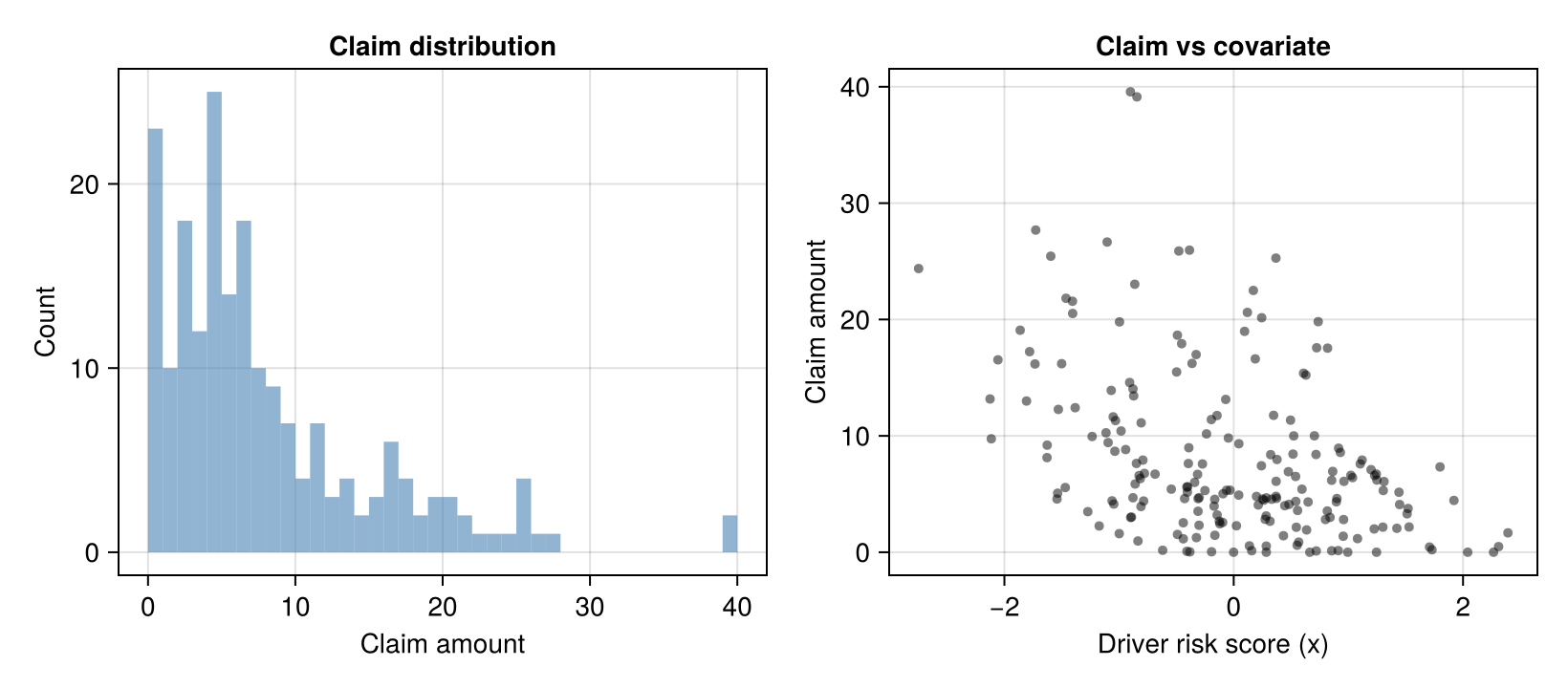

The cluster of zero-claim policies plus the long right tail is the zero-inflated-continuous shape Tweedie was designed for.

The model

The @latte model has the same shape as any other Latte regression: a hyperparameter prior, a Gaussian prior on the regression coefficients, and a ~ statement per observation. The only custom piece is the Tweedie(...) distribution.

We treat the Tweedie power p as a fixed domain choice (p = 1.6 is typical for claim severity). That keeps the hyperparameter dimension at one and focuses the inference on the dispersion φ and the regression coefficients β. To learn p from the data instead, you would add it as another ~ line and Latte would integrate over it as well.

using Latte

@latte function tweedie_glm(y, X, p_fixed)
    φ ~ LogNormal(0.0, 2.0)
    β ~ MvNormal(zeros(size(X, 2)), 100.0 * I(size(X, 2)))
    for i in eachindex(y)
        μ_i = exp(dot(X[i, :], β))
        y[i] ~ Tweedie(μ_i, φ, p_fixed)
    end
end

tweedie_glm (generic function with 1 method)

A few notes on what happens under the hood:

• The custom Tweedie likelihood is not in Latte's fast-path table (Poisson, Bernoulli, Binomial, Normal, NegativeBinomial, Gamma), so the adapter routes it through AutoDiffObservationModel. That covers any logpdf we can write, including ones with an infinite series like Tweedie, at the cost of a little more compile time on the first call.

• We pass likelihood_hessian_pattern = :dense because the Tweedie series expansion is not traceable by SparseConnectivityTracer; the for loop over series terms breaks tracer propagation. For n = 200 a dense Hessian is small, and for very large n you would supply a known sparse pattern explicitly.

• Calling the @latte function returns the LatentGaussianModel. Latte reads φ as a hyperparameter and β as the latent field. Because the prior LogNormal(0, 2) has positive support, the log-transform is inferred automatically and the φ marginal is reported in natural (dispersion) space.

lgm = tweedie_glm(y, X, true_p; likelihood_hessian_pattern = :dense)

LatentGaussianModel
├─ hyperparameters (1)
│    φ  ~ LogNormal(μ=0.0, σ=2.0)  [log]
├─ latent field · 2 dims
│    β  2
└─ likelihood
     custom logpdf · 200 observations

Running INLA

Declaring the prior directly on the natural parameter φ means there is no hyperparameter-derived value for @latte to hoist into the observation payload, so this model runs under the default diff_strategy = ADStrategy() with no extra wiring; the AD path handles a hand-written logpdf without trouble. We pass FiniteDiffStrategy() here as a performance choice: for a custom likelihood with a single hyperparameter, finite differences are about twice as fast as AD on the outer Hessian, and nothing else about the call changes.

result = inla(
    lgm, y;
    diff_strategy = FiniteDiffStrategy(),
    progress = false,
)

INLAResult:
  Model: LatentGaussianModel{HyperparameterSpec{@NamedTuple{φ::Hyperparameter{Base.Fix1{typeof(broadcast), typeof(log)}, :natural}}, @NamedTuple{}}, Latte._PatternAugmentedLatentModel{Latte.RoutedLatentModel{FixedEffectsModel{LinearSolve.DiagonalFactorization, Nothing}, @NamedTuple{}}, SparseArrays.SparseMatrixCSC{Bool, Int64}}, Latte._LiftedSingleObsModel{GaussianMarkovRandomFields.AutoDiffObservationModel{typeof(Main.var"##996".__latte_obs_body_tweedie_glm), ADTypes.AutoForwardDiff{nothing, Nothing}, ADTypes.AutoSparse{ADTypes.AutoForwardDiff{nothing, Nothing}, ADTypes.KnownHessianSparsityDetector{SparseArrays.SparseMatrixCSC{Bool, Int64}}, SparseMatrixColorings.GreedyColoringAlgorithm{:direct, 1, Tuple{SparseMatrixColorings.NaturalOrder}}}, Tuple{Symbol}, typeof(Main.var"##996".__latte_obs_pointwise_tweedie_glm)}, typeof(Main.var"##996".__latte_prelude_tweedie_glm), @NamedTuple{y::Vector{Float64}, X::Matrix{Float64}, p_fixed::Float64}, Tuple{Symbol}, @NamedTuple{β::UnitRange{Int64}}, @NamedTuple{β::Bool}, Tuple{Symbol}}}
  Hyperparameters: 1
  Latent variables: 2
  Mode: (φ=1.5258)
  Convergence: ✓
  Total time: 25.60 seconds
  Exploration: 5 points (5 integration)

Model comparison metrics:
Deviance Information Criterion (DIC):
  DIC: 1214.58
  Effective parameters (p_D): 0.93
  Mean deviance (D̄): 1213.66
  Deviance at mode: 1212.73

Marginal Log-Likelihood:
  log p(y): -619.85

Watanabe-Akaike Information Criterion (WAIC):
  WAIC: 1218.44
  Effective parameters (p_WAIC): 2.69
  Log pointwise predictive density (lppd): -606.53

Conditional Predictive Ordinates (CPO):
  LPML: -602.8
  Mean CPO: 0.063
  Min CPO: 0.0009


Approximation quality (KLD):
  Max SKLD: 0.0000 (variable 1)
  Mean SKLD: 0.0000

Use .hyperparameter_marginals, .latent_marginals, .accumulators for analysis

Posteriors

latent_marginals(result, :β) returns the posterior marginals for the regression coefficients, and hyperparameter_marginals(result, :φ) returns the marginal for φ in natural (dispersion) space, since we declared the prior on φ directly. Each is a Distributions.jl-compatible object, so mean, std, quantile, and the rest work on them directly. summary_df collects the common statistics into a table:

β_summary = summary_df(latent_marginals(result, :β))

2×6 DataFrame
 Row │ mode      median     q2_5       q97_5      mean      std
     │ Float64   Float64    Float64    Float64    Float64   Float64
─────┼────────────────────────────────────────────────────────────────
   1 │  1.9853    1.9853     1.86871    2.10189    1.9853   0.0594443
   2 │ -0.40657  -0.406571  -0.525494  -0.287642  -0.40657  0.0606363

...and the dispersion marginal:

hp_summary = summary_df(hyperparameter_marginals(result, :φ))

1×6 DataFrame
 Row │ mode     median   q2_5     q97_5    mean     std
     │ Float64  Float64  Float64  Float64  Float64  Float64
─────┼───────────────────────────────────────────────────────
   1 │ 1.51307   1.5271  1.32807  1.75723  1.53154  0.111988

Compare to truth:

truth = DataFrame(
    parameter = ["β₁ (intercept)", "β₂ (slope)", "φ"],
    truth = [true_β[1], true_β[2], true_φ],
    posterior_mean = [β_summary.mean[1], β_summary.mean[2], hp_summary.mean[1]],
    q2_5 = [β_summary.q2_5[1], β_summary.q2_5[2], hp_summary.q2_5[1]],
    q97_5 = [β_summary.q97_5[1], β_summary.q97_5[2], hp_summary.q97_5[1]],
)

3×5 DataFrame
 Row │ parameter       truth    posterior_mean  q2_5       q97_5
     │ String          Float64  Float64         Float64    Float64
─────┼───────────────────────────────────────────────────────────────
   1 │ β₁ (intercept)      2.0         1.9853    1.86871    2.10189
   2 │ β₂ (slope)         -0.4        -0.40657  -0.525494  -0.287642
   3 │ φ                   1.5         1.53154   1.32807    1.75723

All three true values land inside the 95% credible intervals. We can also plot the marginal posteriors. Each panel covers a different variable on its own scale, so we assemble a tidy density table from the accessors and facet it, with the true values as a second layer of reference lines:

β_marginals = latent_marginals(result, :β)
φ_marginal = hyperparameter_marginals(result, :φ)[1]

panels = [
    ("β₁ (intercept)", β_marginals[1], true_β[1]),
    ("β₂ (slope)", β_marginals[2], true_β[2]),
    ("φ", φ_marginal, true_φ),
]
density_df = mapreduce(vcat, panels) do (name, marginal, _)
    xs = range(quantile(marginal, 0.001), quantile(marginal, 0.999); length = 200)
    DataFrame(parameter = name, value = xs, density = pdf.(marginal, xs))
end
truth_df = DataFrame(
    parameter = [name for (name, _, _) in panels],
    truth = [true_val for (_, _, true_val) in panels],
)

curves = data(density_df) *
    mapping(:value, :density, layout = :parameter) *
    visual(Lines, color = :steelblue, linewidth = 2)
truth_lines = data(truth_df) *
    mapping(:truth, layout = :parameter) *
    visual(VLines, color = :crimson, linestyle = :dash, linewidth = 2)
draw(curves + truth_lines; facet = (; linkxaxes = :none, linkyaxes = :none))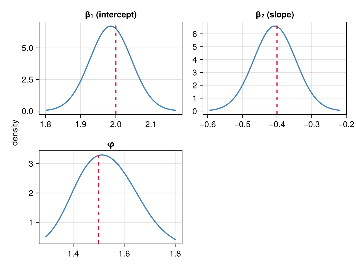

Red dashed lines mark the true values; the posteriors concentrate around them. The dispersion posterior centres on φ ≈ 1.5, the generative truth.

Takeaway

A distribution you can express as logpdf(::MyDist, y) works as an observation likelihood in Latte without any change to the inla() call. The same model shape would carry an ordinal likelihood, a heavy-tailed Student-t, or a Bayesian quantile regression built on the asymmetric Laplace. This fit ran under the default ADStrategy(); we used FiniteDiffStrategy() only as a speed optimisation for the single-hyperparameter outer Hessian.

A few practical tips when writing your own:

• Keep the logpdf AD-friendly. Control flow should branch on y (data, fixed) rather than on the parameters, and avoid Float64-typed buffers in the body; use comprehensions or similar(x, T) so the eltype propagates from the inputs.

• If the logpdf involves an iterative computation (a series, root solver, or ODE solver) that sparsity tracing cannot see through, pass likelihood_hessian_pattern = :dense on the @latte model to skip pattern detection.

• When the likelihood is conditionally independent, which covers most cases, supplying pointwise_loglik_func lets Latte use a faster diagonal-Hessian path. The adapter wires this up automatically; if you build the LatentGaussianModel by hand, pass it to AutoDiffObservationModel yourself.

• ADStrategy() handles the outer hyperparameter gradient for custom likelihoods by default. FiniteDiffStrategy() is a reasonable alternative with only a handful of hyperparameters, where finite differences are cheap and ran somewhat faster here.

For other applications of this pattern, see the rest of the tutorials: hierarchical regressions, smoothing priors, and spatial models.

References

Dunn-Smyth

Series Evaluation of Tweedie Exponential Dispersion Model Densities↗

P. K. Dunn & G. K. Smyth

Statistics and Computing · 2005 · doi:10.1007/s11222-005-4070-y

The numerically stable series expansion of the Tweedie density used here: a log-sum-exp evaluation of the compound Poisson-Gamma infinite series.

Tweedie EDM

Exponential Dispersion Models↗

B. Jørgensen

J. R. Statist. Soc. B · 1987 · doi:10.1111/j.2517-6161.1987.tb01685.x

The exponential-dispersion family that contains the Tweedie distributions, including the compound Poisson-Gamma with power variance function Var[Y] = φ μ^p.

---

This page was generated using Literate.jl.