Handoff: same model, INLA and Turing

Latte uses DynamicPPL's @model macro as its modelling surface. So does Turing.jl. A model you write for inla() can therefore be handed straight to Turing.sample for MCMC, with no rewriting in between.

This tutorial shows the handoff on a small Poisson model with an IID-Normal latent field, and compares the posteriors the two engines return.

The shared model is useful in a few situations:

When you suspect INLA's Laplace approximation might be off on an unusual model, a short NUTS run on the same @model is the most direct check.
INLA is fast and approximate; HMC is slow and asymptotically exact. Keeping one model definition lets you pick the engine per problem.
Latte also exposes hmc_laplace(lgm, y), which runs NUTS over the hyperparameters with an inner Laplace step on the latent field. It sits between inla and full NUTS.

A small Poisson model

julia

using Latte
using DynamicPPL: @model
using Distributions
using GaussianMarkovRandomFields: IIDModel
using Turing
using Random, Statistics
using CairoMakie

Random.seed!(20260424)

@model function iid_poisson(y, n)
    τ ~ PCPrior.Precision(1.0, α = 0.01)
    x ~ IIDModel(n)(τ = τ)
    for i in eachindex(y)
        y[i] ~ Poisson(exp(x[i]); check_args = false)
    end
end

n = 15
true_x = randn(n) .* 0.4 .+ 0.8
y = rand.(Poisson.(exp.(true_x)))
first(y, 5)

5-element Vector{Int64}:
 3
 1
 5
 3
 5

Fit with INLA

latte_from_dppl packages the DPPL model into a LatentGaussianModel that inla() understands. It is the same object tmb() and hmc_laplace() take.

julia

model = iid_poisson(y, n)
lgm = latte_from_dppl(model; random = (:x,))
result = inla(lgm, y; progress = false)

INLAResult:
  Model: LatentGaussianModel{HyperparameterSpec{@NamedTuple{τ::Hyperparameter{Bijectors.TruncatedBijector{Float64, Float64}, :natural}}, @NamedTuple{}}, Latte.CachedDAGLatentModel{Latte.var"#_build_dag_latent##2#_build_dag_latent##3"{DynamicPPL.Model{typeof(Main.var"##976".iid_poisson), (:y, :n), (), (), Tuple{Vector{Int64}, Int64}, Tuple{}, DynamicPPL.DefaultContext, false}, Tuple{Symbol}, @NamedTuple{dims::Dict{Symbol, Int64}, classification::Dict{Symbol, Symbol}, edges::Dict{Symbol, Vector{Symbol}}, is_scalar::Dict{Symbol, Bool}}}, Nothing}, LinearlyTransformedObservationModel{ExponentialFamily{Distributions.Poisson, LogLink, Nothing, Nothing}, SparseArrays.SparseMatrixCSC{Float64, Int64}, Nothing}}
  Hyperparameters: 1
  Latent variables: 15
  Mode: (τ=1.5845)
  Convergence: ✓
  Total time: 12.91 seconds
  Exploration: 5 points (5 integration)

Model comparison metrics:
Deviance Information Criterion (DIC):
  DIC: 48.24
  Effective parameters (p_D): 1.23
  Mean deviance (D̄): 47.0
  Deviance at mode: 45.77

Marginal Log-Likelihood:
  log p(y): -36.64

Watanabe-Akaike Information Criterion (WAIC):
  WAIC: 59.2
  Effective parameters (p_WAIC): 4.68
  Log pointwise predictive density (lppd): -24.92

Conditional Predictive Ordinates (CPO):
  LPML: -1159.65
  Mean CPO: 0.0
  Min CPO: 0.0
  Unreliable observations: 15 / 15
  Max failure score: 49.95
  PIT computed: 15 values
  PIT mean: 0.6344 (ideal: 0.5)


Approximation quality (KLD):
  Max SKLD: 0.0106 (variable 1)
  Mean SKLD: 0.0050

Use .hyperparameter_marginals, .latent_marginals, .accumulators for analysis

Read the latent field back through the accessor, keyed by the name it has in the model (:x), rather than reaching into the result's fields:

julia

x_inla = mean.(latent_marginals(result, :x))
first(x_inla, 5)

5-element Vector{Float64}:
 0.5711840374054646
 0.0
 1.0502608001967144
 0.6450923524346533
 1.0502608001967144

Fit with Turing NUTS

Turing consumes the @model directly, so there is no packaging step here.

julia

chain = sample(model, NUTS(), 2000; progress = false)
x_nuts = [mean(chain[Symbol("x[$i]")]) for i in 1:n];

┌ Info: Found initial step size
└   ϵ = 0.45

Compare posteriors

Latent posterior means from the two engines line up on the diagonal. Raw Makie here: an identity-reference-line scatter (the dashed y = x line spans the shared data range), which AoG's tidy-data idiom does not express cleanly.

julia

fig = Figure(size = (500, 500))
ax = Axis(
    fig[1, 1],
    xlabel = "INLA posterior mean", ylabel = "Turing NUTS posterior mean",
    title = "Latent posterior means (n = $n)"
)
scatter!(ax, x_inla, x_nuts)
lims = extrema(vcat(x_inla, x_nuts))
lines!(ax, [lims...], [lims...], color = :gray, linestyle = :dash)
fig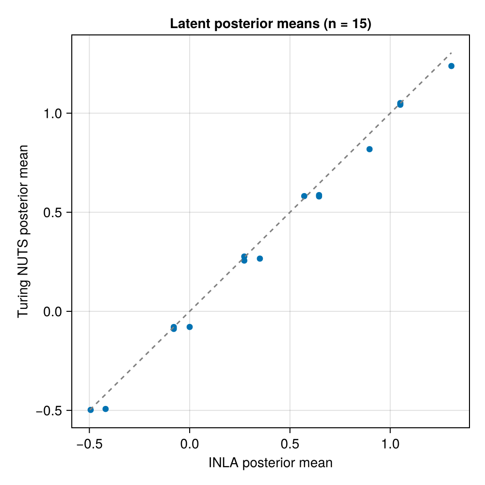

Quantitatively:

julia

println("max |x_INLA − x_NUTS| = ", round(maximum(abs.(x_inla .- x_nuts)), digits = 3))
println("mean |x_INLA − x_NUTS| = ", round(mean(abs.(x_inla .- x_nuts)), digits = 3))

max |x_INLA − x_NUTS| = 0.084
mean |x_INLA − x_NUTS| = 0.037

Caveats

Sharing one @model keeps the specification identical across engines, but a few things are worth knowing before you lean on the comparison:

Constrained GMRF priors (Besag ICAR with sum-to-zero, rank-deficient random walks, and the like) do not sample cleanly under plain NUTS without a reparameterisation onto the constraint manifold. NUTS samples the unconstrained base density and ignores the constraint, which is not the posterior you specified. For a constrained prior, inla(), tmb(), and hmc_laplace() impose the constraint via Kriging conditioning.
Plain NUTS on a latent Gaussian model is usually slower than INLA, since the posterior geometry is awkward for a generic sampler. In practice, run inla() first and turn to hmc_laplace() when you want a sampled hyperparameter posterior.
Heavy tails in hyperparameter marginals (a precision under weak data, say) will differ between the two: INLA extrapolates the tail with a spline, while NUTS only reflects what it visited. Compare medians and credible intervals near the mode, where both are on firm ground.

References

Turing

Turing: A Language for Flexible Probabilistic Inference

H. Ge, K. Xu & Z. Ghahramani

AISTATS (PMLR 84) · 2018

The Turing.jl probabilistic programming language: a flexible Julia system for MCMC-based Bayesian inference. Latte shares its DynamicPPL @model surface, so the same model hands off to Turing.sample.

DynamicPPL

DynamicPPL: Stan-like Speed for Dynamic Probabilistic Models

M. Tarek, K. Xu, M. Trapp, H. Ge & Z. Ghahramani

arXiv preprint · 2020 · arXiv:2002.02702

The modelling-language layer behind Turing and the @model surface Latte builds on: a performant runtime for dynamic probabilistic models.

INLA

Approximate Bayesian Inference for Latent Gaussian Models by Using Integrated Nested Laplace Approximations

H. Rue, S. Martino & N. Chopin

J. R. Statist. Soc. B · 2009 · doi:10.1111/j.1467-9868.2008.00700.x

The original INLA paper: deterministic approximate Bayesian inference for latent Gaussian models via nested Laplace approximations and numerical integration over the hyperparameters.

NUTS

The No-U-Turn Sampler: Adaptively Setting Path Lengths in Hamiltonian Monte Carlo

M. D. Hoffman & A. Gelman

Journal of Machine Learning Research · 2014 · arXiv:1111.4246

The No-U-Turn Sampler, the adaptive Hamiltonian Monte Carlo algorithm Turing's NUTS sampler and Latte's HMC-Laplace engine both run.

Embedded Laplace + HMC

Hamiltonian Monte Carlo using an Adjoint-differentiated Laplace Approximation

C. C. Margossian, A. Vehtari, D. Simpson & R. Agrawal

Advances in Neural Information Processing Systems (NeurIPS) · 2020 · arXiv:2004.12550

Hamiltonian Monte Carlo over the hyperparameters, with the latent Gaussian field marginalised by an embedded Laplace approximation and the gradient propagated through that inner solve. The method Latte's hmc_laplace engine implements.

This page was generated using Literate.jl.

Handoff: same model, INLA and Turing ​

A small Poisson model ​

Fit with INLA ​

Fit with Turing NUTS ​

Compare posteriors ​

Caveats ​

References ​

Handoff: same model, INLA and Turing

A small Poisson model

Fit with INLA

Fit with Turing NUTS

Compare posteriors

Caveats

References