
Disease mapping with spatial models
This tutorial analyzes lung cancer mortality across Pennsylvania counties with the BYM model, estimating disease risk while accounting for spatial correlation between neighboring counties.
What is disease mapping?
Disease mapping estimates disease risk across geographic areas. Crude rates are unstable in areas with small populations, and neighboring areas often share risk through common environmental or socioeconomic factors.
The BYM model (Besag-York-Mollié) is a standard choice for areal data. It splits the county effect into a spatial component (a Besag/ICAR model) for spatially structured variation and an unstructured component (IID) for region-specific deviations.
The Pennsylvania lung cancer dataset
The data record lung cancer mortality across Pennsylvania counties, with observed cases and population broken down by age, race, and gender. That breakdown is what lets us compute expected counts by indirect standardization.
Loading the data:
using CodecBzip2  # needed to decompress .rda files
using RData
using DataFrames
using StatsBase
data_dir = joinpath(@__DIR__, "data")
mkpath(data_dir)
local_rda = joinpath(data_dir, "pennLC_sf.rda")
if !isfile(local_rda)
    repo_url = "https://github.com/rudeboybert/SpatialEpi/raw/refs/heads/master/data/pennLC_sf.rda"
    try
        download(repo_url, local_rda)
    catch err
        error(
            "Could not download dataset (are you offline?). " *
                "Place an RData file at $(local_rda) or pass your own DataFrame."
        )
    end
end

pennLC_sf = load(local_rda)["pennLC_sf"]
first(pennLC_sf, 5)
5×8 DataFrame
Row │ county cases population race gender age smoking geometry
│ String Int32 Int32 Cat… Cat… Cat… Float64 Array…
─────┼───────────────────────────────────────────────────────────────────────────────────────────────
1 │ adams 0 1492 o f Under.40 0.234 [[-77.4467 39.9695; -77.4295 39.…
2 │ adams 0 365 o f 40.59 0.234 [[-77.4467 39.9695; -77.4295 39.…
3 │ adams 1 68 o f 60.69 0.234 [[-77.4467 39.9695; -77.4295 39.…
4 │ adams 0 73 o f 70+ 0.234 [[-77.4467 39.9695; -77.4295 39.…
5 │ adams 0 23351 w f Under.40 0.234 [[-77.4467 39.9695; -77.4295 39.…Preprocessing
We aggregate the data to the county level and add the quantities the model needs:
integer county IDs for the spatial model,
expected counts from indirect standardization (population times the overall rate across all counties),
the standardized incidence ratio (SIR), observed over expected,
and county geometries converted to LibGEOS polygons.
county_data = combine(
    groupby(pennLC_sf, :county),
    :cases => sum => :cases,
    :population => sum => :population,
    :geometry => first => :geometry  # keep geometry for spatial adjacency
)
county_data.county_id = 1:nrow(county_data)
total_cases = sum(county_data.cases)
total_pop = sum(county_data.population)
overall_rate = total_cases / total_pop
county_data.expected = county_data.population .* overall_rate
county_data.SIR = county_data.cases ./ county_data.expected
using LibGEOS
county_data.geometry = [
    LibGEOS.Polygon([[mat[i, :] for i in 1:size(mat, 1)]])
        for mat in county_data.geometry
]
sort!(county_data, :county)
first(county_data, 5)
5×7 DataFrame
Row │ county cases population geometry county_id expected SIR
│ String Int64 Int64 Polygon Int64 Float64 Float64
─────┼────────────────────────────────────────────────────────────────────────────
1 │ adams 55 91292 Polygon(...) 1 76.4096 0.719805
2 │ allegheny 1275 1281666 Polygon(...) 2 1072.73 1.18856
3 │ armstrong 49 72392 Polygon(...) 3 60.5907 0.808705
4 │ beaver 172 181412 Polygon(...) 4 151.838 1.13278
5 │ bedford 37 49984 Polygon(...) 5 41.8356 0.884414The scale of the data:
println("Pennsylvania lung cancer data:")
println("  Counties: ", nrow(county_data))
println("  Total cases: ", total_cases)
println("  Total population: ", total_pop)
println("  Overall rate: ", round(overall_rate * 100000, digits = 2), " per 100,000")
Pennsylvania lung cancer data:
Counties: 67
Total cases: 10279
Total population: 12281054
Overall rate: 83.7 per 100,000SIR summary
Counties with SIR > 1 have higher than expected lung cancer mortality, those with SIR < 1 lower than expected. Mapping the SIR shows the spread across the state.
using AlgebraOfGraphics, CairoMakie
data(county_data) * mapping(:geometry, color = :SIR) * visual(Poly) |> draw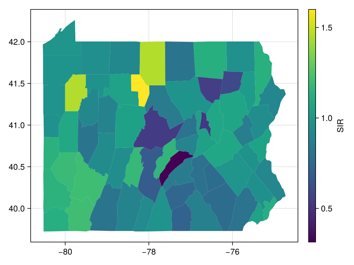
The variability is large: some counties sit well above 1, others well below. The spatial model stabilizes these estimates by borrowing strength from neighboring counties.
The BYM model
For each county i we model the observed cases as
The Besag model needs an adjacency structure that says which counties are neighbors. GaussianMarkovRandomFields.jl builds a contiguity-based adjacency matrix from the county geometries:
using GaussianMarkovRandomFields, SparseArrays
geom_collection = LibGEOS.GeometryCollection(county_data.geometry)
W = contiguity_adjacency(geom_collection)
size(W), nnz(W) ÷ 2  # counties and number of shared borders
((67, 67), 173)We write the BYM model as an @latte block with three latent pieces. The intercept β is a one-element MvNormal, which gives the adapter a simple random-effect structure to recognise. The spatial component spatial ~ BesagModel(W; …)(τ = τ_besag) returns a ConstrainedGMRF: BesagModel enforces a sum-to-zero constraint per connected component of the adjacency graph, which keeps the intercept identified from the spatial field. The unstructured component is u ~ IIDModel(n)(τ = τ_iid).
using Latte
using Distributions
using LinearAlgebra
n = nrow(county_data)

@latte function bym_model(cases, expected, n, W)
    τ_besag ~ PCPrior.Precision(1.0, α = 0.01)
    τ_iid ~ PCPrior.Precision(1.0, α = 0.01)
    β ~ MvNormal(zeros(1), 100.0 * I(1))
    spatial ~ BesagModel(W; normalize_var = Val{true}())(τ = τ_besag)
    u ~ IIDModel(n)(τ = τ_iid)
    for i in eachindex(cases)
        cases[i] ~ Poisson(
            expected[i] * exp(β[1] + spatial[i] + u[i])
        )
    end
end
bym_model (generic function with 1 method)Prior specification
Both precisions get PC (Penalized Complexity) priors, which favor the simpler model unless the data pull away from it. PCPrior.Precision(1.0, α = 0.01) calibrates that preference as
Running INLA
The expected exposure enters the likelihood through expected[i] * exp(…), which the adapter picks up as a log-exposure offset automatically.
lgm = bym_model(county_data.cases, county_data.expected, n, W)
inla_result = inla(lgm, county_data.cases; progress = false)
INLAResult:
Model: LatentGaussianModel{HyperparameterSpec{@NamedTuple{τ_besag::Hyperparameter{Bijectors.TruncatedBijector{Float64, Float64}, :natural}, τ_iid::Hyperparameter{Bijectors.TruncatedBijector{Float64, Float64}, :natural}}, @NamedTuple{}}, Latte._PatternAugmentedLatentModel{Latte.RoutedLatentModel{CombinedModel{LinearSolve.CHOLMODFactorization{Nothing}}, @NamedTuple{τ_besag::Symbol, τ_iid::Symbol}}, SparseArrays.SparseMatrixCSC{Int64, Int64}}, LinearlyTransformedObservationModel{ExponentialFamily{Distributions.Poisson, LogLink, Nothing, Nothing}, SparseArrays.SparseMatrixCSC{Float64, Int64}, Vector{Float64}}}
Hyperparameters: 2
Latent variables: 135
Mode: (τ_besag=118.6602, τ_iid=115.9855)
Convergence: ✓
Total time: 16.67 seconds
Exploration: 16 points (16 integration)
Model comparison metrics:
Deviance Information Criterion (DIC):
DIC: 453.87
Effective parameters (p_D): 1.93
Mean deviance (D̄): 451.94
Deviance at mode: 450.02
Marginal Log-Likelihood:
log p(y): -281.68
Watanabe-Akaike Information Criterion (WAIC):
WAIC: 504.6
Effective parameters (p_WAIC): 18.22
Log pointwise predictive density (lppd): -234.08
Conditional Predictive Ordinates (CPO):
LPML: -265.71
Mean CPO: 0.0325
Min CPO: 0.0
PIT computed: 67 values
PIT mean: 0.4839 (ideal: 0.5)
Approximation quality (KLD):
Max SKLD: 0.0129 (variable 1)
Mean SKLD: 0.0002
Use .hyperparameter_marginals, .latent_marginals, .accumulators for analysisThis returns posterior marginals for every parameter.
Hyperparameter posteriors
The two precision parameters summarize how much spatial and unstructured variation the model attributes to the data:
summary_df(hyperparameter_marginals(inla_result))2×6 DataFrame
Row │ mode median q2_5 q97_5 mean std
│ Float64 Float64 Float64 Float64 Float64 Float64
─────┼──────────────────────────────────────────────────────
1 │ 79.7189 117.467 46.4104 314.759 134.24 70.1231
2 │ 83.4562 125.758 54.7949 391.399 150.225 87.9429Evaluating each marginal density on its own grid gives a tidy frame we can hand to AlgebraOfGraphics, faceted by component:
function density_frame(dist, label)
    grid = range(quantile(dist, 0.001), quantile(dist, 0.999); length = 200)
    return DataFrame(τ = grid, density = pdf.(Ref(dist), grid), component = label)
end
hyper_density = vcat(
    density_frame(hyperparameter_marginals(inla_result, :τ_besag)[1], "Spatial (τ_besag)"),
    density_frame(hyperparameter_marginals(inla_result, :τ_iid)[1], "Unstructured (τ_iid)"),
)
data(hyper_density) *
    mapping(:τ => "Precision", :density => "Posterior density", layout = :component) *
    visual(Lines) |> draw(; facet = (; linkxaxes = :none))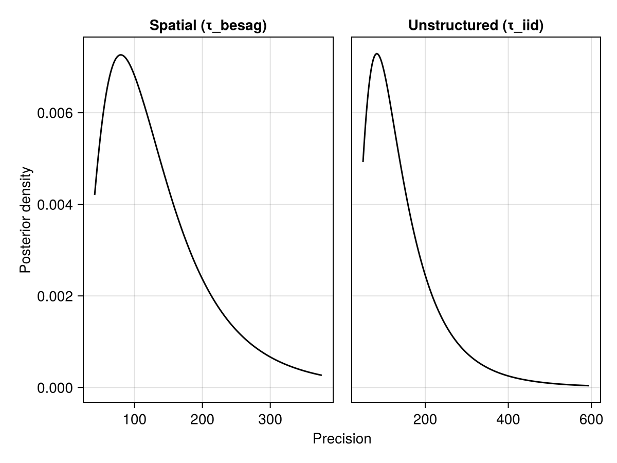
Visualizing the latent spatial and unstructured effects
Before turning to relative risk, it helps to look at the model components directly. The BYM model splits each county's effect into a spatial part (shared with neighbors) and an unstructured part (county-specific). These base latent marginals are the building blocks that combine into the linear predictor.
base_latent_marginals(result) returns them in the order the variables appear in the model body: β, then spatial, then u. Index 1 is β, indices 2:(1+n) are the spatial effects, and the next n are u.
n_counties = nrow(county_data)
spatial_offset = 1
iid_offset = 1 + n_counties
base_marginals = base_latent_marginals(inla_result)
length(base_marginals) # β (1) + spatial (n) + u (n)135A joyplot shows how these effects vary across a selection of counties:
sorted_idx = sortperm(county_data.SIR, rev = true)
component_indices = vcat(
    sorted_idx[1:3],              # 3 highest SIR
    sorted_idx[33:35],            # 3 middle SIR
    sorted_idx[(end - 2):end]
)        # 3 lowest SIR

spatial_dists = [base_marginals[spatial_offset + i] for i in component_indices]
spatial_labels = [county_data.county[i] * " (spatial)" for i in component_indices]
iid_dists = [base_marginals[iid_offset + i] for i in component_indices]
iid_labels = [county_data.county[i] * " (IID)" for i in component_indices]
9-element Vector{String}:
"cameron (IID)"
"potter (IID)"
"venango (IID)"
"susquehanna (IID)"
"lawrence (IID)"
"montgomery (IID)"
"centre (IID)"
"montour (IID)"
"juniata (IID)"Raw Makie: joyplot! is Latte's ridgeline recipe for marginal objects; AlgebraOfGraphics has no equivalent and cannot consume opaque distributions directly.
fig_components = Figure(size = (1200, 600))
ax_spatial = Axis(
    fig_components[1, 1],
    title = "Spatial Component (Besag)",
    xlabel = "Effect",
    ylabel = ""
)
ax_iid = Axis(
    fig_components[1, 2],
    title = "Unstructured Component (IID)",
    xlabel = "Effect",
    ylabel = ""
)
joyplot!(
    ax_spatial, spatial_dists;
    labels = spatial_labels,
)
joyplot!(
    ax_iid, iid_dists;
    labels = iid_labels,
)
fig_components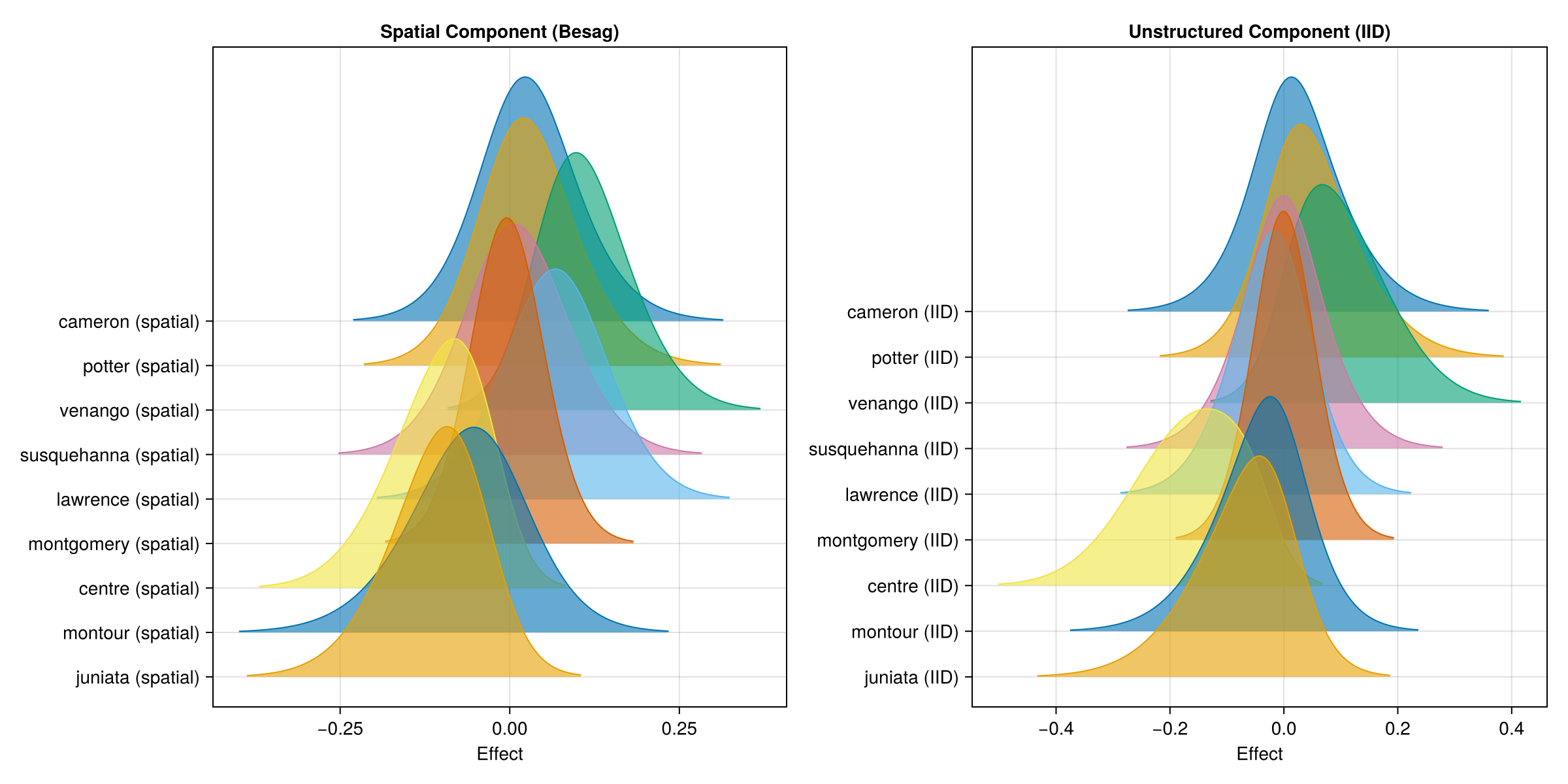
The spatial component varies smoothly and is shared between neighboring counties, while the IID component captures county-specific deviations. The spatial effects sit in tighter distributions because the spatial structure regularizes them; the IID effects vary more freely. This is the separation of smooth spatial signal from local noise that the BYM model is built to do.
Posterior relative risk estimates
The quantity of interest is the relative risk for each county. observation_marginals returns marginals of the fitted count
obs_marginals = observation_marginals(inla_result)
fitted_summary = summary_df(obs_marginals)
risk_summary = DataFrame(
    county = county_data.county,
    SIR = county_data.SIR,
    median = fitted_summary.median ./ county_data.expected,
    mean = fitted_summary.mean ./ county_data.expected,
    q2_5 = fitted_summary.q2_5 ./ county_data.expected,
    q97_5 = fitted_summary.q97_5 ./ county_data.expected,
    geometry = county_data.geometry,
)
first(select(risk_summary, :county, :SIR, :median, :q2_5, :q97_5), 10)
10×5 DataFrame
Row │ county SIR median q2_5 q97_5
│ String Float64 Float64 Float64 Float64
─────┼───────────────────────────────────────────────────
1 │ adams 0.719805 0.787186 0.651563 0.943893
2 │ allegheny 1.18856 1.1802 1.11861 1.24529
3 │ armstrong 0.808705 0.941603 0.783422 1.11406
4 │ beaver 1.13278 1.11304 0.97937 1.26566
5 │ bedford 0.884414 0.918921 0.757393 1.1096
6 │ berks 0.984883 0.965938 0.873945 1.06896
7 │ blair 1.17494 1.06319 0.919491 1.23712
8 │ bradford 1.12317 1.01448 0.849802 1.21848
9 │ bucks 0.907621 0.917967 0.842351 0.999819
10 │ butler 1.08439 1.07011 0.94317 1.21407Comparing smoothed vs crude estimates
Overlaying the crude SIR and the smoothed posterior estimate on a shared county axis shows what the spatial model buys us. The posterior layer carries its 95% credible interval as range bars:
risk_summary.county_id = 1:nrow(risk_summary)
risk_layers =
    mapping(:county_id => "County", :q2_5, :q97_5) *
    visual(Rangebars, color = (:steelblue, 0.3), whiskerwidth = 0) +
    mapping(:county_id => "County", :SIR => "Risk ratio", color = direct("Crude SIR")) *
    visual(Scatter, markersize = 6) +
    mapping(
    :county_id => "County", :median => "Risk ratio",
    color = direct("Posterior median (BYM)"),
) * visual(Scatter, markersize = 8)
draw(
    data(risk_summary) * risk_layers;
    axis = (title = "Crude SIR vs posterior relative risk",),
)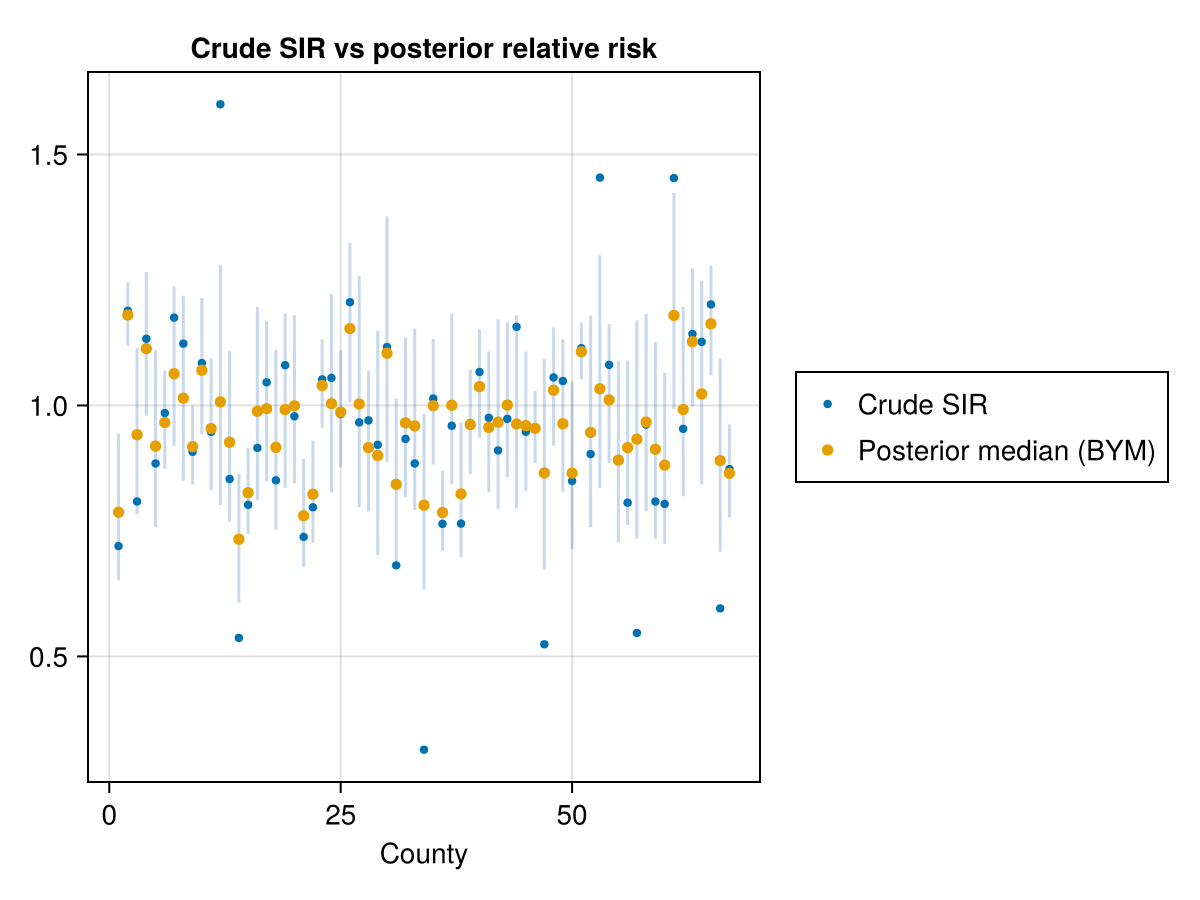
The posterior estimates are more stable than the crude SIRs. Extreme values shrink toward 1.0, spatial smoothing pulls neighboring counties toward similar estimates, and the 95% credible intervals quantify the remaining uncertainty.
Visualizing posterior distributions with joyplots
Credible intervals report two numbers; a joyplot shows the full posterior. Picking the 5 highest- and 5 lowest-risk counties brings out how the distributions differ.
The fitted-count marginals live on the county-specific count scale, so their densities span very different widths (a county with thousands of cases has a much flatter density than one with fifty). Stacked as-is, every ridge would be nearly flat. Dividing each marginal by its expected count puts all of them on the common relative-risk scale, where the curves are comparable and legible. pushforward carries the full distribution through the Y_i / E_i map, not just its summaries:
using Bijectors: Scale
sorted_by_risk = sortperm(risk_summary.median, rev = true)
selected_indices = vcat(
    sorted_by_risk[1:5],      # 5 highest risk
    sorted_by_risk[(end - 4):end]
) # 5 lowest risk

selected_dists = [
    pushforward(obs_marginals[i], Scale(1.0 / county_data.expected[i]))
        for i in selected_indices
]
selected_labels = [county_data.county[i] for i in selected_indices]

fig_joy = joyplot(
    selected_dists;
    labels = selected_labels,
    title = "Posterior relative-risk distributions (selected counties)",
    xlabel = "Relative risk",
)
fig_joy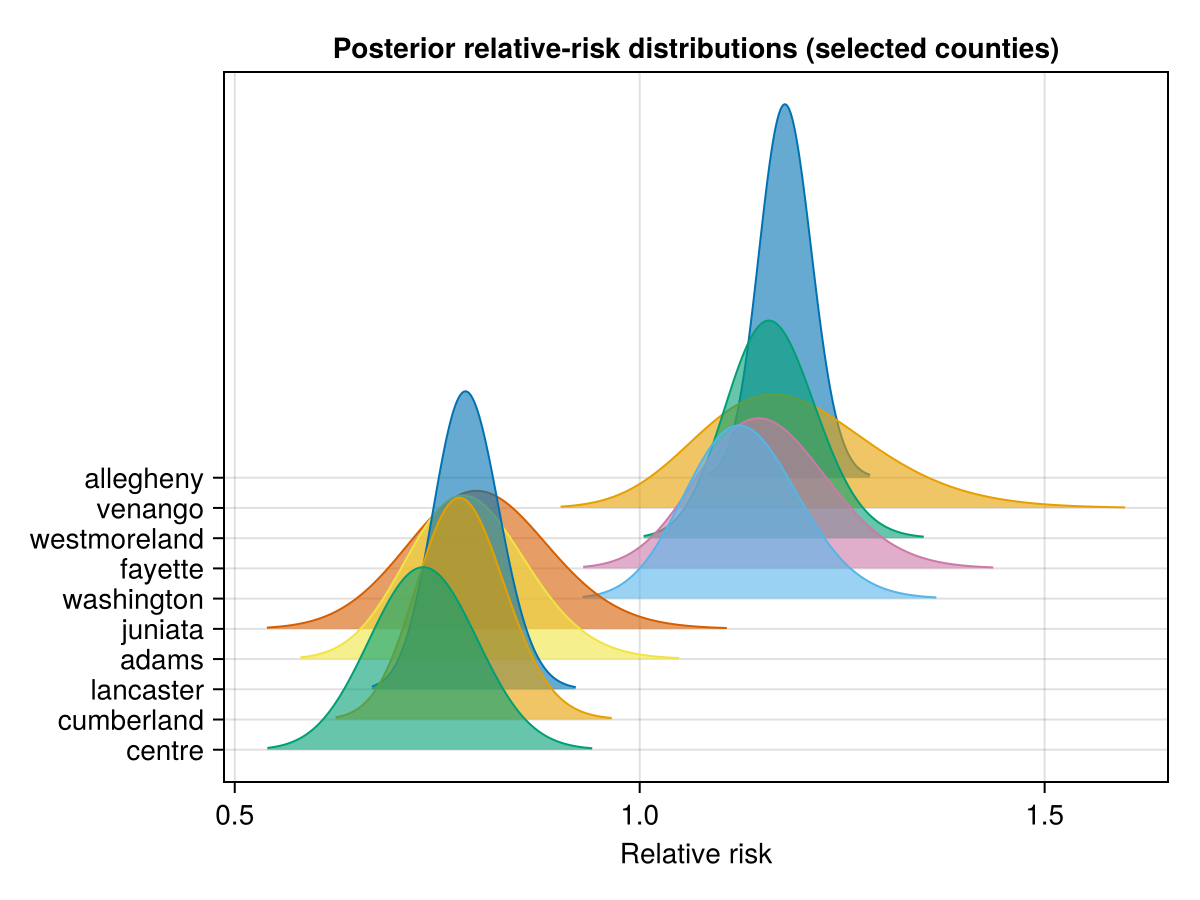
The high-risk counties have relative-risk distributions sitting above 1.0, the low-risk counties below it. The width of each distribution reflects uncertainty: counties with smaller populations have wider, less certain distributions.
Identifying high-risk counties
A county shows significantly elevated risk when its entire 95% credible interval lies above 1.0:
high_risk = risk_summary[
    risk_summary.q2_5 .> 1.0,
    [:county, :median, :q2_5, :q97_5],
]
4×4 DataFrame
Row │ county median q2_5 q97_5
│ String Float64 Float64 Float64
─────┼─────────────────────────────────────────
1 │ allegheny 1.1802 1.11861 1.24529
2 │ fayette 1.15312 1.00629 1.32418
3 │ philadelphia 1.1069 1.05155 1.16522
4 │ westmoreland 1.16265 1.05963 1.2779Reduced risk is the mirror image: the whole interval below 1.0.
low_risk = risk_summary[
    risk_summary.q97_5 .< 1.0,
    [:county, :median, :q2_5, :q97_5],
]
10×4 DataFrame
Row │ county median q2_5 q97_5
│ String Float64 Float64 Float64
─────┼──────────────────────────────────────────
1 │ adams 0.787186 0.651563 0.943893
2 │ bucks 0.917967 0.842351 0.999819
3 │ centre 0.733372 0.607121 0.86379
4 │ chester 0.826186 0.74456 0.915271
5 │ cumberland 0.780285 0.678722 0.893286
6 │ dauphin 0.823057 0.726741 0.929739
7 │ juniata 0.801232 0.632957 0.983221
8 │ lancaster 0.78658 0.710408 0.869524
9 │ lebanon 0.82374 0.69829 0.965915
10 │ york 0.86478 0.777366 0.962296Exceedance probabilities
For each county we can compute the probability that relative risk exceeds a threshold, say 1.1 for 10% elevated risk. The marginals are on the fitted-count scale, so
threshold = 1.1
risk_summary.exc_prob = [
    1 - cdf(obs_marginals[i], threshold * county_data.expected[i])
        for i in 1:nrow(risk_summary)
]
data(risk_summary) * mapping(:geometry, color = :exc_prob) * visual(Poly) |> draw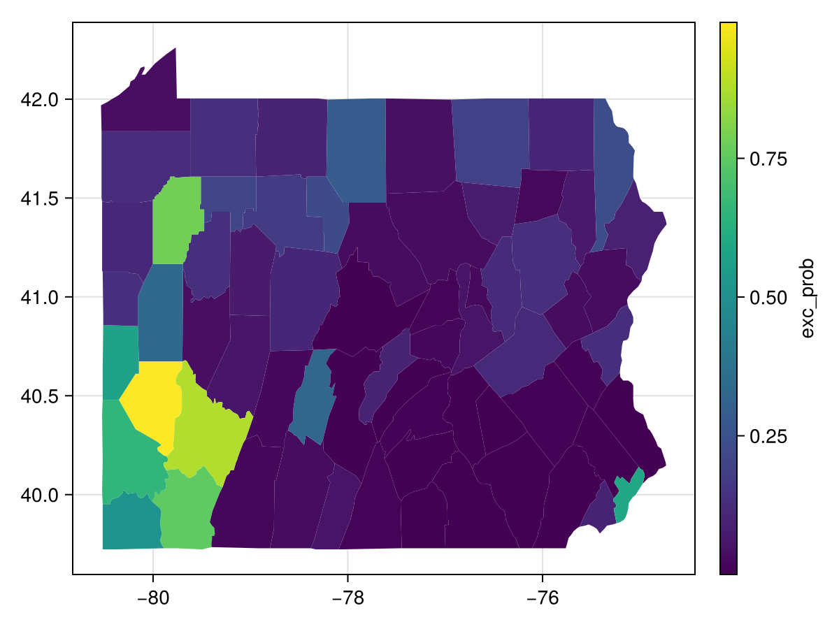
The counties where that probability exceeds 0.95:
risk_summary[
    risk_summary.exc_prob .> 0.95,
    [:county, :median, :exc_prob],
]
1×3 DataFrame
Row │ county median exc_prob
│ String Float64 Float64
─────┼──────────────────────────────
1 │ allegheny 1.1802 0.994974Model diagnostics and comparison
The default accumulators report the DIC (with its effective parameter count p_D) and the log marginal likelihood. To judge whether the spatial component earns its place, we fit a second model with only unstructured random effects:
@latte function iid_only(cases, expected, n)
    τ_iid ~ PCPrior.Precision(1.0, α = 0.01)
    β ~ MvNormal(zeros(1), 100.0 * I(1))
    u ~ IIDModel(n)(τ = τ_iid)
    for i in eachindex(cases)
        cases[i] ~ Poisson(expected[i] * exp(β[1] + u[i]))
    end
end

lgm_iid = iid_only(county_data.cases, county_data.expected, n)
inla_result_iid = inla(lgm_iid, county_data.cases; progress = false)
INLAResult:
Model: LatentGaussianModel{HyperparameterSpec{@NamedTuple{τ_iid::Hyperparameter{Bijectors.TruncatedBijector{Float64, Float64}, :natural}}, @NamedTuple{}}, Latte._PatternAugmentedLatentModel{Latte.RoutedLatentModel{CombinedModel{LinearSolve.CHOLMODFactorization{Nothing}}, @NamedTuple{τ_iid::Symbol}}, SparseArrays.SparseMatrixCSC{Int64, Int64}}, LinearlyTransformedObservationModel{ExponentialFamily{Distributions.Poisson, LogLink, Nothing, Nothing}, SparseArrays.SparseMatrixCSC{Float64, Int64}, Vector{Float64}}}
Hyperparameters: 1
Latent variables: 68
Mode: (τ_iid=51.5808)
Convergence: ✓
Total time: 10.90 seconds
Exploration: 5 points (5 integration)
Model comparison metrics:
Deviance Information Criterion (DIC):
DIC: 445.08
Effective parameters (p_D): 0.67
Mean deviance (D̄): 444.4
Deviance at mode: 443.73
Marginal Log-Likelihood:
log p(y): -283.71
Watanabe-Akaike Information Criterion (WAIC):
WAIC: 501.17
Effective parameters (p_WAIC): 18.25
Log pointwise predictive density (lppd): -232.33
Conditional Predictive Ordinates (CPO):
LPML: -271.44
Mean CPO: 0.0315
Min CPO: 0.0001
PIT computed: 67 values
PIT mean: 0.485 (ideal: 0.5)
Approximation quality (KLD):
Max SKLD: 0.0107 (variable 1)
Mean SKLD: 0.0007
Use .hyperparameter_marginals, .latent_marginals, .accumulators for analysisPutting the two fits side by side:
DataFrame(
    model = ["BYM (spatial + unstructured)", "IID only"],
    DIC = round.(
        [inla_result.accumulators[1].DIC, inla_result_iid.accumulators[1].DIC],
        digits = 2,
    ),
    p_D = round.(
        [inla_result.accumulators[1].p_D, inla_result_iid.accumulators[1].p_D],
        digits = 2,
    ),
    log_ML = round.(
        [
            inla_result.accumulators[2].log_marginal_likelihood,
            inla_result_iid.accumulators[2].log_marginal_likelihood,
        ],
        digits = 2,
    ),
)
2×4 DataFrame
Row │ model DIC p_D log_ML
│ String Float64 Float64 Float64
─────┼─────────────────────────────────────────────────────────
1 │ BYM (spatial + unstructured) 453.87 1.93 -281.68
2 │ IID only 445.08 0.67 -283.71A lower DIC and higher marginal likelihood for the BYM model would indicate that the data carry spatial structure the IID model cannot capture.
Summary
We started from raw Pennsylvania lung cancer counts and used the BYM model to separate spatial pattern from noise. Borrowing strength across neighboring counties produced more stable risk estimates than the crude SIRs, which matters most where populations are small.
The spatial component captured smooth geographic variation and the unstructured component the county-specific deviations. Looking at the full posteriors through joyplots showed how uncertainty changes across the risk spectrum, and exceedance probabilities turned the posteriors into direct statements about which counties are likely above a given risk threshold.
The BYM model is a standard tool in spatial epidemiology for count data over small areas where neighboring regions are expected to be similar.
To go further, see Getting started with Latte.jl for the INLA basics, or the main documentation for how hyperparameter priors work.
References
Introduces the Besag-York-Mollié model: an areal count model combining a spatially structured intrinsic CAR effect with an unstructured IID effect, the standard decomposition for disease mapping.
The foundational paper on conditional autoregressive (CAR) models, the intrinsic Gaussian Markov random field that the spatial component of the BYM model is built from.
Penalised Complexity priors shrink each model component toward a simpler base model, with interpretable scaling such as P(σ > U) = α; the priors used on both BYM precisions here.
This page was generated using Literate.jl.